
The pursuit of high-speed helicopter technology has driven the development of advanced transmission architectures. Among these, transmission systems employing herringbone gears are recognized for their high efficiency and smooth operational characteristics, presenting significant application potential. However, the inherent imperfections in manufacturing and assembly processes introduce errors that prevent perfectly uniform load distribution among power branches in split-torque configurations. This non-uniform load sharing critically impacts the static and dynamic load-sharing characteristics, ultimately influencing the overall reliability and service life of the entire transmission system. Therefore, analyzing and understanding load-sharing behavior is paramount in the design of gear-based power-split systems. This study focuses on a coaxial counter-rotating transmission system utilizing herringbone gears for its final output stage. We establish a detailed static analysis model that comprehensively incorporates transmission chain stiffness, bearing support stiffness, manufacturing errors, and alignment errors. Through the derivation of system torque equilibrium equations and deformation compatibility conditions, we systematically investigate the influence mechanism of various error types—both individually and in combination—on the system’s static load-sharing performance. The findings aim to provide a foundational reference for the structural design and performance optimization of such complex transmission systems.
1. Introduction and System Configuration
The coaxial counter-rotating herringbone gear transmission system represents a sophisticated solution for applications requiring two concentric output shafts rotating at equal speed but in opposite directions, such as helicopter main rotors. The specific system configuration analyzed in this work is illustrated schematically. It consists of a three-stage gear train designed to split, redirect, and recombine power flow efficiently.
The system comprises the following key components:
- Stage I: An input helical pinion (Z1) meshing with a helical gear (Z2). This stage serves as the primary speed reduction and torque multiplication step.
- Stage II (Differential/Reversal Stage): This stage facilitates power split and direction reversal. The torque from gear Z2 is transmitted via two parallel shafts to two identical small bevel gears (Z3, Z4). Each of these meshes with a larger bevel gear (Z5, Z6), effecting a 90-degree change in the power flow direction and creating two independent power paths.
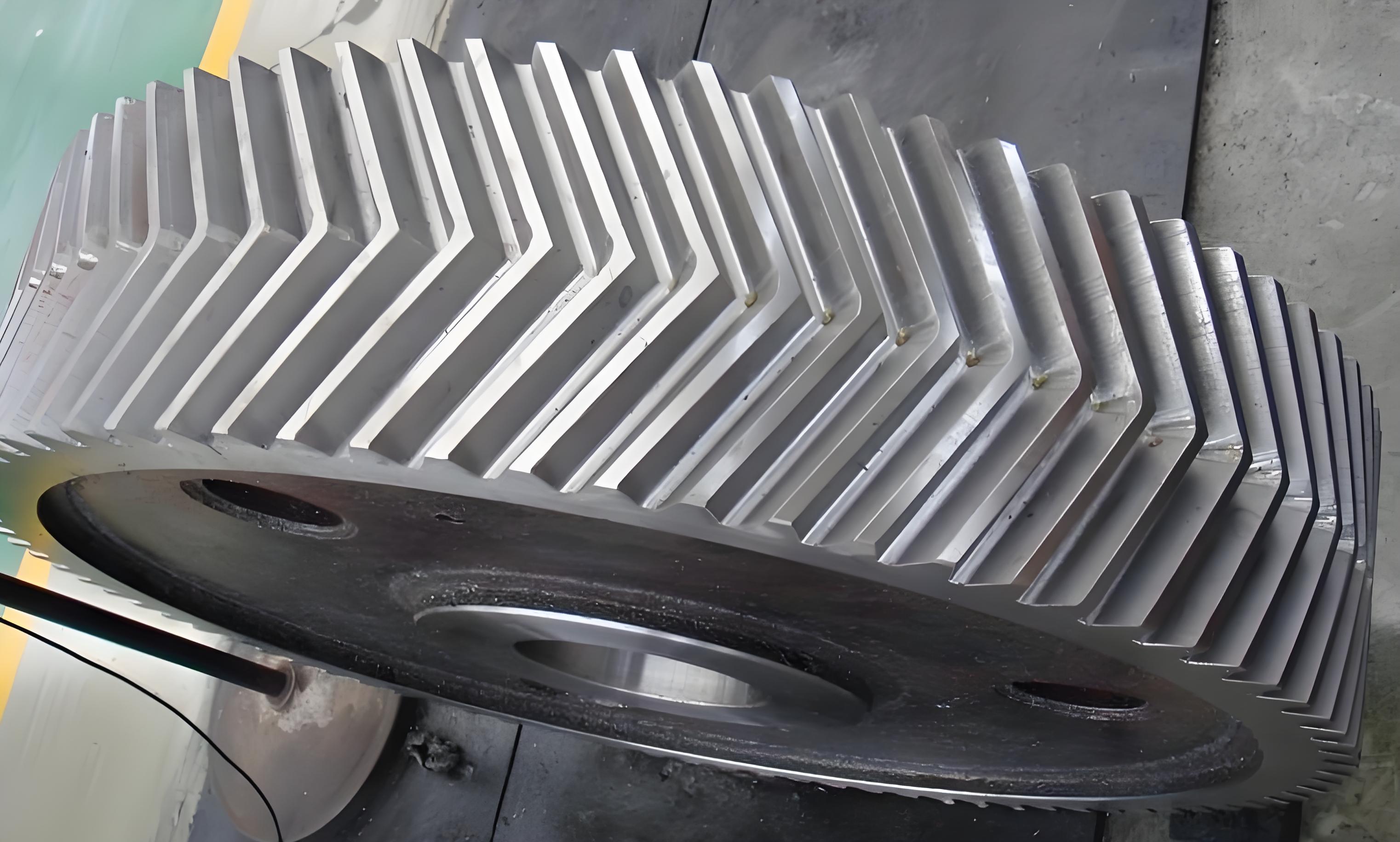
- Stage III (Herringbone Output Stage): This is the critical power-combining stage featuring herringbone gears. The output from bevel gear Z5 drives a small herringbone gear Z7, which meshes with a large output herringbone gear Z9. Similarly, the output from bevel gear Z6 drives small herringbone gear Z8, which meshes with large output herringbone gear Z10. Gears Z9 and Z10 are mounted on concentric output shafts, with the lower rotor shaft passing through the center of the upper rotor shaft. The symmetrical but opposite helix angles of the herringbone gears inherently balance axial thrust and provide smooth, high-torque transmission to the counter-rotating outputs.
The power from the single input is thus divided into two parallel paths (Path A: Z1-Z2-Z3-Z6-Z8-Z10; Path B: Z1-Z2-Z4-Z5-Z7-Z9) before being recombined at the two output shafts. The fundamental challenge is to ensure that these two paths share the load equally under realistic conditions involving component errors and system compliance.
2. Theoretical Modeling for Static Analysis
To analyze the static load-sharing characteristics, a lumped-parameter model is developed based on the following key assumptions:
- Gear bodies, shafts (except for their torsional flexibility), and housings are modeled as rigid components.
- Gear mesh interfaces, shaft torsional segments, and bearing supports are modeled as linear springs, characterized by their respective stiffness values.
- Effects of friction, thermal expansion, and dynamic inertial forces are neglected for this static analysis.
- All errors (manufacturing, alignment) are treated as static displacements projected onto the line of action of each gear mesh.
2.1 System Torque Equilibrium Equations
The internal torque transmission within the system is defined. Let \( T_{i\_j} \) represent the torque transmitted from gear \( i \) to gear \( j \). Defining input torque as positive and load torque as negative, the static torque balance for the entire system can be established. After simplification, an independent system of equations with five unknown torques is obtained:
$$
\begin{cases}
T_{in} – T_{1\_2} = 0 \\
-T_{1\_2} \cdot \eta_{1\_2} + T_{3\_6} + T_{4\_5} = 0 \\
-T_{3\_6} \cdot \eta_{3\_6} + T_{8\_10} = 0 \\
-T_{4\_5} \cdot \eta_{4\_5} + T_{7\_9} = 0
\end{cases}
$$
where \( T_{in} \) is the input torque, \( \eta_{i\_j} \) is the transmission ratio from gear \( i \) to \( j \), and \( T_{1\_2}, T_{3\_6}, T_{4\_5}, T_{7\_9}, T_{8\_10} \) are the key internal torques to be solved.
Furthermore, considering the elastic support provided by bearings, force equilibrium equations must be established for each gear shaft in the transverse (x, y) directions. For any gear \( i \) involved in meshes, the sum of mesh force components must balance the bearing reaction forces:
$$
\begin{cases}
\sum \left[ \frac{T_{i\_j}}{r_{bi} \cos \alpha_n} \cdot \cos \lambda_{i\_j} \right] – K_{xi} x_i = 0 \\
\sum \left[ \frac{T_{i\_j}}{r_{bi} \cos \alpha_n} \cdot \sin \lambda_{i\_j} \right] – K_{yi} y_i = 0
\end{cases}
$$
where \( x_i \) and \( y_i \) are the translational displacements of gear \( i \) in the x and y directions, \( K_{xi} \) and \( K_{yi} \) are the corresponding bearing support stiffnesses, \( r_{bi} \) is the base radius of gear \( i \), \( \alpha_n \) is the normal pressure angle, and \( \lambda_{i\_j} \) is the angle between the line of action for mesh \( i\_j \) and the x-axis.
2.2 Deformation Compatibility Conditions
The system’s compliance and errors determine how the total input torque is divided between the two parallel paths. The relative angular displacement at the meshing point between gear \( i \) and \( j \), denoted \( \delta_{i\_j} \), consists of several components.
First, the relative torsional displacement due to shaft flexibility is:
$$
\delta_{t_{i\_j}}(T_{i\_j}) = \frac{T_{i\_j}}{K_{t_{i\_j}}}
$$
where \( K_{t_{i\_j}} \) is the torsional stiffness of the shaft segment between the two components.
Second, the comprehensive mesh error \( \delta_{w_i} \), which is the projection of both manufacturing and alignment errors onto the line of action, is given by:
$$
\delta_{w_i} = \delta_{e_i} + \delta_{a_i} = E_i \sin(\alpha_n + \beta_{e_i} + \omega_i t) + A_i \sin(\alpha_n + \beta_{a_i})
$$
where \( E_i \) and \( A_i \) are the amplitudes of manufacturing and alignment errors, respectively, \( \beta_{e_i} \) and \( \beta_{a_i} \) are their corresponding phase angles, \( \omega_i \) is the angular velocity, and \( t \) is time. For static analysis, the time-varying term related to manufacturing error (e.g., eccentricity) is evaluated at a specific instance or treated as a static offset.
Third, the relative angular displacement caused by the translational movement of gear centers (due to bearing compliance) is:
$$
\delta_{C_{i\_j}} = \frac{[(x_i – x_j) \cos \Xi_{i\_j} + (y_i – y_j) \sin \Xi_{i\_j}]}{r_{bi}}
$$
where \( \Xi_{i\_j} \) is the angle between the line of action for mesh \( i\_j \) and the x-axis.
The total equivalent angular displacement error at a mesh point is the sum of the compliance-induced displacement and the geometric error:
$$
\delta_{S_{i\_j}} = \delta_{C_{i\_j}} + \delta_{w_i}
$$
Finally, the total transmission error \( \delta_{i\_j} \) for a gear pair, incorporating the elastic deflection due to the mesh force itself, is expressed as:
$$
\delta_{i\_j} = \frac{T_{i\_j}}{K_{i\_j} \cdot r_i \cdot r_{bi} \cos \alpha_n} + \delta_{S_{i\_j}}
$$
where \( K_{i\_j} \) is the mesh stiffness of gear pair \( i\_j \), and \( r_i \) is the operating pitch radius.
The deformation compatibility condition requires that the sum of all relative angular displacements (transmission errors) around any closed loop in the system must be zero. Considering the two primary power paths (A and B), the following compatibility equations are derived:
$$
\begin{aligned}
&\delta_{1\_2} + \eta_{1\_2}\delta_{2\_3} + \eta_{1\_2}\delta_{3\_6} + \eta_{1\_2}\eta_{3\_6}\delta_{6\_8} + \eta_{1\_2}\eta_{3\_6}\delta_{8\_10} = \delta_1 – \eta_{1\_2}\eta_{3\_6}\eta_{8\_10}\delta_{10} \\
&\delta_{1\_2} + \eta_{1\_2}\delta_{2\_3} + \eta_{1\_2}\delta_{3\_4} + \eta_{1\_2}\delta_{4\_5} + \eta_{1\_2}\eta_{4\_5}\delta_{5\_7} + \eta_{1\_2}\eta_{4\_5}\delta_{7\_9} = \delta_1 – \eta_{1\_2}\eta_{4\_5}\eta_{7\_9}\delta_{9}
\end{aligned}
$$
These equations, coupled with the torque and force equilibrium equations, form a complete set of nonlinear algebraic equations. Solving this system yields the internal load distribution \( T_{i\_j} \) under the influence of stiffness parameters and error inputs.
3. Methodology and System Parameters
3.1 Load Sharing Coefficient Definition
To quantitatively evaluate the uniformity of load distribution, static load-sharing coefficients are defined for the two output branches. The coefficient for a branch is the ratio of the actual calculated torque in that branch to its ideal, theoretically equal share of the total output torque.
$$
\Omega_U = \frac{\max(T_{8\_10})}{T’_{8\_10}}, \quad \Omega_L = \frac{\max(T_{7\_9})}{T’_{7\_9}}
$$
where \( \Omega_U \) and \( \Omega_L \) are the load-sharing coefficients for the upper and lower output herringbone gear pairs, respectively. \( T’_{i\_j} \) is the ideal torque calculated solely based on the total power and speed ratio. A perfectly uniform system would have \( \Omega_U = \Omega_L = 1 \). Values greater than 1 indicate that the corresponding branch is carrying more than its fair share of the load, which is detrimental to system reliability.
3.2 Baseline System Data
The analysis is performed using a realistic set of parameters for a high-power transmission system. The operating conditions and key geometric parameters for the herringbone gears and other stages are listed below.
Operating Conditions: Input Power \( P = 1400 \text{ kW} \), Input Speed \( n = 9000 \text{ rpm} \).
| Gear Stage | Gear Designation | Number of Teeth | Normal Module (mm) | Pressure Angle (°) | Helix/Spiral Angle (°) |
|---|---|---|---|---|---|
| Stage I | Input Pinion Z1 | 25 | 3 | 20 | 11 (Helical) |
| Stage I | Gear Z2 | 70 | 3 | 20 | 11 (Helical) |
| Stage II | Small Bevel Gears Z3, Z4 | 30 | 5 | 20 | 15 (Spiral) |
| Stage II | Large Bevel Gears Z5, Z6 | 70 | 5 | 20 | 30 (Spiral) |
| Stage III | Small Herringbone Gears Z7, Z8 | 22 | 5 | 20 | 30 (Herringbone) |
| Stage III | Large Herringbone Gears Z9, Z10 | 120 | 5 | 20 | 30 (Herringbone) |
| Mesh Stiffness | Value (N/m) | Torsional Stiffness | Value (N·m/rad) |
|---|---|---|---|
| \( K_{1\_2} \) | 1.85 × 10⁹ | \( K_{t_{2\_3}} \) | 2.04 × 10⁷ |
| \( K_{3\_6}, K_{4\_5} \) | 1.95 × 10⁹ | \( K_{t_{3\_4}} \) | 1.145 × 10⁷ |
| \( K_{7\_9}, K_{8\_10} \) | 2.35 × 10⁹ | \( K_{t_{5\_6}} \) | 3.74 × 10⁵ |
| – | – | \( K_{t_{6\_8}} \) | 3.237 × 10⁵ |
| Bearing Location (Gear) | Radial Stiffness, Kx, Ky (N/m) |
|---|---|
| Z1 | 1.45 × 10⁹ |
| Z2 | 1.48 × 10⁹ |
| Z3, Z4 | 1.34 × 10⁹ |
| Z5, Z6 | 5.14 × 10⁹ |
| Z7, Z8 | 1.98 × 10⁹ |
| Z9, Z10 | 7.01 × 10⁹ |
4. Analysis of Error Effects on Load-Sharing Performance
Using the established model and parameters, a series of analyses are conducted to isolate and understand the impact of different error types on the load-sharing coefficients \( \Omega_U \) and \( \Omega_L \).
4.1 Influence of Manufacturing Errors
We first examine the effect of manufacturing errors (e.g., eccentricity) acting on specific gear sets. The error amplitude is varied from 0 μm to 50 μm.
Case 1: Stage II Small Bevel Gears (Z3 & Z4). When manufacturing errors on gears Z3 and Z4 increase simultaneously, the load-sharing coefficients show a distinct trend. The lower output branch coefficient \( \Omega_L \) initially decreases from 1.10 to 1.02 before rising to 1.23, marking a net increase of 10.6%. The upper output branch coefficient \( \Omega_U \) increases monotonically from 1.10 to 1.45, a significant increase of 24.1%. The initial decrease in \( \Omega_L \) suggests that for small error magnitudes (0-15 μm), the introduced error can partially compensate for the inherent load imbalance caused by system stiffness variations. Beyond this threshold, the manufacturing error dominates and exacerbates the non-uniformity.
Case 2: Stage III Small Herringbone Gears (Z7 & Z8). The impact of errors on the herringbone gears in the final, power-combining stage is more pronounced. As the manufacturing error on Z7 and Z8 increases simultaneously, both \( \Omega_U \) and \( \Omega_L \) rise sharply. \( \Omega_U \) increases by 50%, reaching 1.65, while \( \Omega_L \) increases by 43.3%, reaching 1.58. This demonstrates the high sensitivity of the system’s load distribution to errors in the final meshes where the power streams converge.
From a design tolerance perspective, to maintain load-sharing within a typical ±5% margin (\( \Omega \leq 1.05 \)), the following manufacturing error limits can be inferred:
- For Stage II bevel gears (Z3, Z4): Simultaneous errors should be maintained within approximately 5-25 μm.
- For Stage III small herringbone gears (Z7, Z8): Simultaneous errors require tighter control, ideally within a narrow band around 5 ±2 μm.
4.2 Influence of Alignment Errors
Alignment errors (e.g., shaft misalignment) are investigated next, with amplitude also varied from 0 to 50 μm.
Case 1: Stage II Small Bevel Gears (Z3 & Z4). The effect of alignment errors in this stage is less severe than manufacturing errors. As errors increase, \( \Omega_U \) first slightly decreases to 1.01 then rises to 1.08. \( \Omega_L \) shows a complementary, symmetric variation. The system can tolerate alignment errors in Z3/Z4 between 10-50 μm while keeping both \( \Omega_U \) and \( \Omega_L \) within the 1.05 limit.
Case 2: Stage III Small Herringbone Gears (Z7 & Z8). Similar to manufacturing errors, alignment errors in the final stage herringbone gears have a strong effect. \( \Omega_U \) increases from 1.10 to 1.46 (a 24.7% increase), and \( \Omega_L \) follows a symmetric, opposite trend. This confirms that the final meshing stage, particularly the small herringbone gears, is a critical control point for system performance.
4.3 Influence of Comprehensive Errors
In reality, multiple errors exist simultaneously on different components. We analyze the effect of a “comprehensive error” (an aggregate of manufacturing and alignment errors) applied individually to key gears. The results highlight the relative importance of different gear positions.
| Gear with Error | Max \( \Omega_U \) | Increase in \( \Omega_U \) | Max \( \Omega_L \) | Critical Error Range for Ω ≤ 1.05 |
|---|---|---|---|---|
| Z3 (Stage II Bevel) | 1.15 | 4.5% | 1.23 | ~5-25 μm |
| Z8 (Stage III Herringbone) | 1.80 | 38.9% | 1.42 | ~5-15 μm |
| Z9 (Stage III Herringbone) | 1.75 | 37.3% | 1.40 | ~5-15 μm |
| Z10 (Stage III Herringbone) | 1.78 | 38.0% | 1.41 | ~5-15 μm |
The analysis reveals a clear hierarchy of sensitivity:
- Gear Z8 (Small Herringbone in Path A): This component has the single greatest influence on system load-sharing. A comprehensive error of 50 μm causes \( \Omega_U \) to surge by 38.9%, indicating a severe overloading of its branch.
- Gears Z9 & Z10 (Large Output Herringbone Gears): These gears also show very high sensitivity, with error-induced increases in \( \Omega_U \) around 37-38%.
- Gear Z3 (Stage II Bevel Gear): Errors at this earlier stage in the power path have a comparatively muted effect, causing a maximum increase of only 4.5% in \( \Omega_U \).
The non-monotonic behavior of \( \Omega_L \), which often decreases initially before rising, is consistently observed. This is attributed to the complex interaction between the introduced error and the system’s elastic deformation field, where small errors can sometimes improve balance by counteracting other inherent asymmetries.
4.4 Influence of Operating Speed Under Error Conditions
While the analysis is static, the model incorporates speed-dependent terms for manufacturing errors like eccentricity (\( \omega_i t \)). By evaluating the system at different rotational speeds, we can observe the coupling effect of speed and error. The speed is varied from 7,000 rpm to 15,000 rpm, concurrent with introducing manufacturing errors on specific gears.
Case with Error on Z3: At a constant speed of 13,000 rpm, \( \Omega_U \) increases with error. For a fixed error of 25 μm on Z3, as speed increases from 7,000 to 15,000 rpm, \( \Omega_U \) grows from 1.17 to 1.25, and \( \Omega_L \) increases from 1.03 to 1.05.
Case with Error on Z8: The effect is more dramatic. For a fixed error of 10 μm on the critical herringbone gear Z8, increasing speed from 7,000 to 15,000 rpm leads to a significant rise in \( \Omega_U \). Similarly, \( \Omega_L \) initially benefits from a slight compensatory effect at low error and speed but then deteriorates.
The general trend is unequivocal: increasing system rotational speed amplifies the detrimental effect of gear errors on load-sharing uniformity. Higher speeds effectively increase the magnitude of the oscillatory component of manufacturing errors projected onto the mesh line of action, leading to greater instantaneous load imbalance. This underscores the necessity for stricter error control in high-speed applications of herringbone gear transmission systems.
5. Conclusion
This study presents a comprehensive static analysis of load-sharing characteristics in a coaxial counter-rotating transmission system, with particular emphasis on the critical role of the final herringbone gear stage. By developing a detailed model that integrates transmission stiffness, bearing compliance, and various gear errors, we have derived and solved the system’s equilibrium and compatibility equations to quantify load distribution.
The key conclusions are as follows:
- Sensitivity to Error Type and Location: The system’s load-sharing performance is highly sensitive to errors, particularly those occurring in the Stage III herringbone gears. Manufacturing or alignment errors on the small herringbone gears (Z7, Z8) can increase the load-sharing coefficient by up to 50% and 24.7%, respectively. Errors in the preceding bevel gear stage (Z3, Z4) have a less severe but still significant impact.
- Critical Component Identification: Under the action of comprehensive errors, gear Z8 (the small herringbone gear in one power path) is identified as the most influential component, causing the upper branch load-sharing coefficient \( \Omega_U \) to increase by 38.9%. This pinpoints a critical area for precision control during manufacturing and assembly.
- Non-Linear and Compensatory Effects: The relationship between error magnitude and load-sharing is not always linear. For certain components and branches (notably the lower output branch \( \Omega_L \)), small errors can initially improve load distribution by compensating for stiffness-induced imbalances. However, beyond a small threshold, larger errors consistently degrade performance.
- Speed-Error Coupling: Increased operational speed exacerbates the negative impact of gear errors on load-sharing uniformity. This coupling effect mandates even tighter tolerances for high-speed applications of these herringbone gear systems.
Engineering Significance: The findings provide clear guidance for the design and manufacturing of helicopter main reducers and similar coaxial counter-rotating transmissions. To effectively enhance system reliability and longevity through improved load-sharing:
- Tightest tolerances must be allocated to the final power-combining herringbone gear meshes, especially the small herringbone pinions (Z7, Z8).
- Control of comprehensive error (the combined effect of manufacturing and alignment) is more critical than focusing on any single error type in isolation.
- System performance should be verified across the entire operational speed envelope, as high-speed conditions present the greatest challenge to uniform load distribution.
Future work will extend this model to dynamic analysis, incorporating time-varying mesh stiffness and inertial effects to predict dynamic load factors and system vibration response under error conditions.