
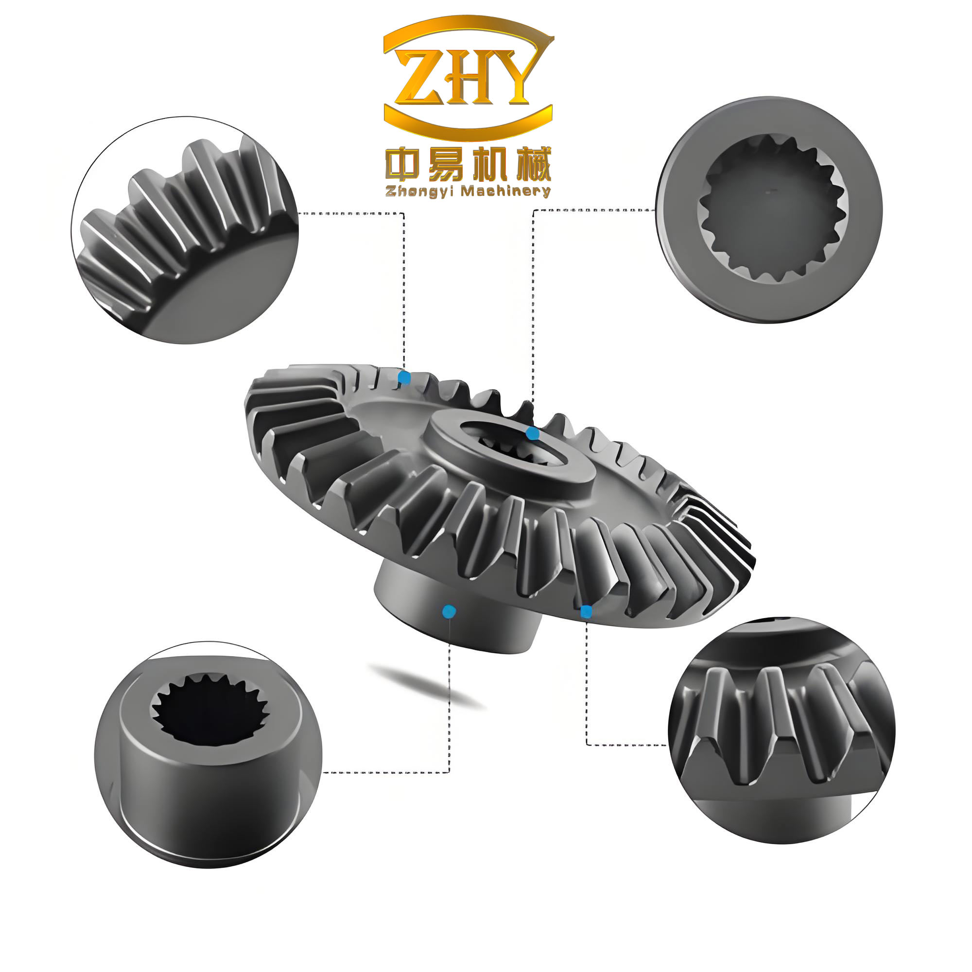
Straight bevel gears are widely used in mechanical transmissions that require power transfer between intersecting axes. Their manufacturing simplicity and low cost make them attractive for automotive, machine tool, and general industrial applications. However, the nominal line-contact meshing of a straight bevel gear pair is highly sensitive to assembly errors and elastic deflections, often causing edge loading, stress concentration, vibration, and noise. Tooth modification is an efficient way to improve the meshing quality of such gears. In this research, I investigate modification methods for the tooth surfaces of straight bevel gears with a common profile generated by a planing process. The work covers the theoretical generation of modified tooth surfaces, tooth contact analysis (TCA), finite element static contact analysis, and computer numerical control (CNC) machining simulation. Throughout the study, the focus is on the straight bevel gear, its modification geometry, and its performance under load.
1. Generation of the Unmodified Straight Bevel Gear Tooth Surface
The straight bevel gear studied here is produced by the traditional planing process based on a crown gear with a flat top. The tool cutting edges are straight, and the generating motion is equivalent to a plane enveloping the gear tooth. To derive the tooth surface equation, I set up the coordinate systems shown in the classical generation model. The machine coordinate system \(\mathcal{S}_m\) is fixed, with its origin at the center of the cradle. The cradle coordinate system \(\mathcal{S}_g\) rotates about the \(z_m\)-axis. The auxiliary system \(\mathcal{S}_a\) is attached to the cradle and shifted by a distance \(E\) to locate the tool position. The tool system \(\mathcal{S}_c\) is offset by the pressure angle \(\alpha\) from the auxiliary system. The workgear system \(\mathcal{S}_b\) is rotated by the dedendum angle \(\delta_f\), and the gear system \(\mathcal{S}_1\) rotates with the workpiece.
In the basic case, the cutting edge generates a plane in the tool coordinate system. The generating surface can be expressed in \(\mathcal{S}_c\) as:
$$
\mathbf{r}_c(l,d) = \begin{bmatrix} d \\ 0 \\ l \\ 1 \end{bmatrix}, \qquad
\mathbf{n}_c = \begin{bmatrix} 0 \\ 1 \\ 0 \\ 1 \end{bmatrix}
$$
where \(d\) and \(l\) are surface parameters. The transformation from the tool system to the gear system is given by:
$$
\mathbf{M}_{c1}(\phi,\varphi) = \mathbf{M}_{b1}(\varphi)\mathbf{M}_{mb}\mathbf{M}_{gm}(\phi)\mathbf{M}_{ag}\mathbf{M}_{ca}
$$
with the rotation angle of the cradle \(\phi\) and the workpiece rotation \(\varphi = I_f \phi\). The machine ratio \(I_f\) is constant for an unmodified gear:
$$
I_f = \frac{\cos\theta}{\sin\delta}
$$
where \(\theta\) is the root angle and \(\delta\) is the pitch angle. The meshing condition between the generating surface and the gear tooth is:
$$
f(l,d,\phi) = \mathbf{n}_m \cdot \mathbf{v}_m = 0
$$
Solving the meshing equation together with the position vector yields the unmodified tooth surface \(\mathbf{r}_1(l,d)\) and its normal \(\mathbf{n}_1(l,d)\).
2. Modification of the Straight Bevel Gear Tooth Surface
2.1 Axial (longitudinal) modification
To obtain a localized contact pattern, the cutting tool is made to move along a parabolic trajectory on the cradle plane. Instead of a straight radial line, the tool path is described in the auxiliary system as:
$$
\mathbf{r}_c^{\text{par}}(l,d) = \begin{bmatrix} d \\ a d^2 \\ l \\ 1 \end{bmatrix}
$$
The generating surface becomes a parabolic cylinder. Its unit normal is:
$$
\mathbf{n}_c^{\text{par}} = \frac{1}{\sqrt{1+4a^2d^2}} \begin{bmatrix} -2ad \\ 1 \\ 0 \\ 1 \end{bmatrix}
$$
The parameter \(a\) controls the amount of lengthwise crowning, while the parameter \(E\) in the coordinate shift matrix control the location of the crowning apex. I set the apex at the midface through \(E = R_e – b/2\), where \(R_e\) is the outer cone distance and \(b\) is the face width. This lengthwise modification converts the theoretical line contact into a point contact, greatly reducing the sensitivity to misalignment.
2.2 Profile modification
Profile modification is achieved by varying the roll ratio between the cradle and the workpiece during generation. The instantaneous roll ratio is:
$$
I_f(\phi) = \frac{\cos\theta}{\sin\delta} + 2b(\phi+\phi_0)
$$
Here \(b\) is the profile modification coefficient and \(\phi_0\) controls the location of the profile crowning. The tool remains straight, so the generating surface is still a plane. This modification controls the amplitude and symmetry of the transmission error curve without changing the line-contact nature.
2.3 Combined modification
For simultaneous longitudinal and profile modification, both the parabolic tool trajectory and the variable roll ratio are applied. The generating surface is the parabolic cylinder, and the meshing condition now includes the modified roll ratio. The resulting tooth surface has a local convexity in both the lengthwise and height directions, providing a point contact with a favorable transmission error curve.
2.4 Calculation and visualization of the deviation
To evaluate the modification amount, I define a grid on the axial plane of the gear. For each projected grid point \((X_j, Y_j)\), the corresponding point on the unmodified surface \(P_j^0\) and on the modified surface \(P_j\) are found by solving:
$$
x_j = X_j, \qquad \sqrt{y_j^2+z_j^2} = Y_j
$$
The normal deviation is then:
$$
\delta_j = \pm \sqrt{(x_j-x_j^0)^2+(y_j-y_j^0)^2+(z_j-z_j^0)^2}
$$
with the sign determined by whether the modified point lies below or above the unmodified surface. I used a gear with \(Z_1=32\), \(Z_2=37\), module \(m=2.5\) mm, pressure angle \(\alpha=20^\circ\), axis angle \(90^\circ\) to compute the deviation maps. Table 1 summarizes the maximum deviation values for the three modification strategies.
| Modification type | Maximum deviation (μm) | Position |
|---|---|---|
| Axial (longitudinal) | 19 | Toe/root area |
| Profile | 46 | Toe/tip area |
| Combined | 40 | Tip area |
The deviation maps showed zero modification at the crowning point, increasing gradually toward the edges, which confirms the desired “crowning” effect along both directions.
3. Tooth Contact Analysis (TCA) of the Straight Bevel Gear
I formulated the TCA using the fixed frame \(\mathcal{S}_f\). The pinion is attached to \(\mathcal{S}_1\), and the gear to \(\mathcal{S}_2\). The axis angle is \(\gamma = 90^\circ\). The surfaces are transformed into the common fixed frame. For point contact, the positions and normals satisfy:
$$
\mathbf{r}_f^{(1)}(l_1,d_1,\vartheta_1) = \mathbf{r}_f^{(2)}(l_2,d_2,\vartheta_2), \qquad
\mathbf{n}_f^{(1)}(l_1,d_1,\vartheta_1) = \mathbf{n}_f^{(2)}(l_2,d_2,\vartheta_2)
$$
where \(\vartheta_1\) and \(\vartheta_2\) are the rotation angles of the pinion and gear, respectively. This vector equation yields five independent scalar equations for six unknowns. Taking \(\vartheta_1\) as the input, I solved the system by Newton’s method in MATLAB to obtain the contact path and the transmission error.
For line-contact simulations (when no axial modification is applied), an additional condition is required to select a particular point on the instantaneous contact line. I chose the point at the midface width:
$$
l_1 = R_e – \frac{b}{2}
$$
This condition provides a well-posed system for the line-contact case.
Table 2 lists the parameters of the straight bevel gear pair used in the TCA and finite element analyses.
| Parameter | Value |
|---|---|
| Pinion teeth \(Z_1\) | 32 |
| Gear teeth \(Z_2\) | 37 |
| Module \(m\) | 2.5 mm |
| Pressure angle \(\alpha\) | 20° |
| Addendum coefficient | 1 |
| Dedendum coefficient | 0.2 |
| Shaft angle \(\gamma\) | 90° |
For the unmodified pair, the transmission error curve was parabolic with a maximum of about 60 seconds over a rotation cycle of 40 degrees. The contact pattern extended along the full face width, a typical line-contact characteristic. When only the pinion was axially modified (\(a=0.0002\)), the contact became localized, with an elliptical footprint, but the transmission error remained essentially unchanged because axial modification does not affect the kinematic mismatch. For profile-only modification (\(b=0.002\), \(\phi_0=0.018\)), the line contact remained, but the transmission error amplitude reduced to about 3 seconds per degree, and the error curve became nearly symmetric. For the combined modification, the gear pair achieved point contact and the transmission error amplitude was reduced to the same low level as the profile-only case. These results confirm that the combination of axial and profile modification gives both a localized contact pattern and a smooth, low-amplitude transmission error curve.
4. Finite Element Static Contact Analysis
4.1 Finite element model generation
The finite element mesh of the straight bevel gear was generated directly from the tooth surface equation, avoiding the need for a CAD solid model. I wrote a MATLAB program to compute the nodal coordinates of the tooth surfaces, then interpolated the interior nodes through the tooth thickness direction. The gear body was truncated to the web area, and only three teeth were modeled for each gear to reduce computational cost. I used eight-node SOLID45 elements. The nodes on the tooth surfaces were arranged with 14 layers along the tooth height, 19 layers along the face width, and 4 layers along the thickness, yielding 2160 nodes and 1292 elements per tooth.
The pinion and gear meshes were directly generated in the assembly coordinate system using the position obtained from the TCA program. Therefore, no additional coordinate transformation was needed when importing the model into ANSYS. The assembled three-teeth contact model is illustrated in the previous figure conceptually. Figure 4-3 from the original work is not reproduced here for brevity; instead, I emphasize that the assembly was automatically positioned.
4.2 Contact definition and boundary conditions
Three contact pairs were created between the pinion and gear teeth. The gear tooth surfaces were taken as the target surfaces (TARGE170), and the pinion tooth surfaces as the contact surfaces (CONTA174). The coefficient of friction was set to zero, assuming no influence of friction on the static contact stress. The normal contact stiffness factor FKN was set to 1.0, and the penetration tolerance FTOLN to 0.1. The meshing process was simulated at seven discrete positions within one engagement cycle.
Boundary conditions were applied as follows: the inner nodes of the gear rim and two side faces of the non-central gear teeth were fully constrained. For the pinion, a mass point element MASS21 at the pitch apex was rigidly connected to the inner rim and side faces. All translational degrees of freedom of this point were restrained except the rotation around the pinion axis. A driving torque of \(M = 100\ \mathrm{N\cdot m}\) was applied to the mass point.
4.3 Results and discussion
I calculated the von Mises stress distribution for the pinion and gear tooth surfaces at each meshing position for four cases: unmodified, axial modification only, profile modification only, and combined modification. The maximum contact stress values on the pinion are listed in Table 3, and those on the gear in Table 4 for the seven positions.
| Position | 1 | 2 | 3 | 4 | 5 | 6 | 7 |
|---|---|---|---|---|---|---|---|
| Unmodified | 53.93 | 137 | 131.68 | 263 | 124.62 | 128.93 | 51.82 |
| Axial mod. | 112.46 | 183.70 | 203.12 | 262.1 | 228.23 | 196.70 | 102.71 |
| Profile mod. | 205.13 | 100.36 | 163.51 | 261.78 | 159.2 | 132.75 | 210.08 |
| Combined mod. | 205.13 | 106.94 | 163.26 | 261.78 | 137.82 | 128.18 | 109.36 |
| Position | 1 | 2 | 3 | 4 | 5 | 6 | 7 |
|---|---|---|---|---|---|---|---|
| Unmodified | 38.25 | 127.62 | 129.33 | 254.38 | 130.07 | 105.24 | 58.36 |
| Axial mod. | 106.15 | 187.12 | 229.64 | 295.66 | 213.41 | 184.24 | 116.33 |
| Profile mod. | 80.12 | 105.07 | 147.62 | 251.84 | 139.26 | 121.65 | 163.01 |
| Combined mod. | 205.26 | 184.23 | 169.28 | 269.05 | 195.55 | 194.98 | 137.54 |
For the unmodified gear pair, the contact area was a long thin band along the tooth length, and the stress was unevenly distributed with pronounced edge concentrations at the toe and heel. The maximum stress on both members occurred at the single-tooth contact position (position 4). After axial modification, the contact pattern became an ellipse, eliminating the edge stress concentrations. However, because the same torque was concentrated on a smaller area, the peak stress increased compared to the unmodified case. For example, at position 4 the pinion stress was 262.1 MPa versus 263 MPa for the unmodified; at other positions the increase was more evident. Profile modification did not change the line-contact nature, so edge loading persisted. The combined modification also produced an elliptical contact pattern and reduced the peak stress compared to axial-only modification at most positions. From Table 3, the maximum pinion stress for the combined case at position 4 is 261.78 MPa, which is slightly lower than the 263 MPa of the unmodified case. This indicates that with carefully chosen modification parameters, it is possible to maintain a comparable stress level while improving the load distribution and reducing edge contact.
5. Three-Dimensional Modeling and CNC Machining Simulation
5.1 Solid model construction in UG
I generated the precise 3D model of the straight bevel gear using the tooth surface data computed in MATLAB. The surface points were imported into UG NX 6.0, and the “Through Points” command created a single tooth flank. The symmetric flank was obtained by mirroring. A ruled surface was built for the bottom of the tooth space, and then the surfaces were stitched together. The face cone was created by rotating the tip line about the gear axis. Finally, the tooth space was subtracted from the face cone and the resulting single tooth space was arrayed to produce the complete gear model. This method ensures the 3D solid model exactly matches the modified tooth surface equation.
5.2 CNC machining simulation
To verify that the modified tooth surface can be produced by CNC machining, I used the manufacturing module of UG NX 6.0. A fixture was prepared with the gear blank and the same workpiece coordinate system used for modeling. The machining sequence for one tooth space included:
- Rough milling with a flat end mill of diameter 1 mm. The cut region was the two tooth flanks and the bottom surface. The cutting mode was reciprocal, with step over 20% of the tool diameter and the part stock 1 mm.
- Semi-finish milling with a ball end mill of diameter 1 mm. The stock was 0.5 mm, step over 10% of the tool diameter, and the milling direction was changed to up-cut for better surface quality.
- Finish milling of the flanks with the same ball end mill. The stock was 0 mm, step over 5% of the tool diameter, and the flanks were selected as the cut region.
- Finish milling of the bottom with the same parameters, using the bottom surface as the cut region.
- Clean-up milling along the concave edges to remove any remaining material.
The generated tool paths were checked by simulated cutting. The simulation showed that the modified tooth surface could be accurately machined. The step-over values were small enough to represent the smooth modification surface. This proves the feasibility of using a multi-axis CNC machine to produce modified straight bevel gear tooth surfaces, even though the traditional planing process cannot easily realize the complex modification.
6. Concluding Remarks and Future Work
In this research, I presented a complete methodology for the design, analysis, and machining simulation of modified straight bevel gears. The main conclusions are:
- The tooth surface of a straight bevel gear with a common profile can be represented mathematically using the planing generation model. Axial modification is realized by giving the tool a parabolic motion path, while profile modification is realized by a variable roll ratio. The combined modification provides both longitudinal and profile crowning.
- TCA results show that axial modification changes the line contact to point contact without affecting the transmission error; profile modification reduces the amplitude and improves the symmetry of the transmission error while retaining line contact. Combining both modifications yields point contact and a favorable transmission error curve simultaneously.
- The finite element contact analysis indicates that unmodified straight bevel gears suffer from edge loading and stress concentration. Axial modification eliminates edge contacts but slightly raises the peak stress. Profile modification alone does not remove edge loading. Combined modification offers the best compromise, with a localized elliptical contact and manageable peak stress.
- The direct generation of the finite element mesh from the tooth surface equation saves time and improves accuracy compared to CAD-based mesh generation. The APDL scripts automate the model import, contact definition, and boundary condition setup.
- The solid CAD model and the CNC machining simulation demonstrate that the modified tooth surface can be produced by a generic multi-axis milling process, making the proposed modification practical for manufacturing.
Future work may include the consideration of alignment errors and elastic tooth deflections in TCA, the use of loaded tooth contact analysis (LTCA) to optimize modification parameters under realistic loads, and the extension of the same generation approach to spiral bevel gears. The fabrication and experimental testing of the modified straight bevel gear pair would be the next logical step to validate the numerical findings.