
Herringbone gears are widely used in automotive, aerospace, marine and mining machinery due to their compact structure, negligible axial force, high load-carrying capacity and excellent transmission efficiency. In high-speed and heavy-load applications, the microscopic morphology of tooth surfaces plays a critical role in the lubrication state and power loss of gear meshing. In this work, I focus on the external meshing pair of an aero-engine herringbone gear planetary transmission system. I combine dynamic modeling and simulation analysis to investigate the effects of manufacturing precision, input speed and realistic surface micro-topography on the lubrication state and frictional power loss. I then apply a genetic algorithm in a gear simulation environment to optimize the tooth surface modification, aiming at improving meshing efficiency and reducing power dissipation. The research covers dynamic modeling, mixed lubrication friction coefficient, real surface measurement, and tooth profile modification. Extensive tables and formulas are provided to illustrate the theoretical derivations and simulation results.
1. Introduction and Research Background
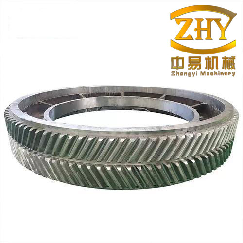
Herringbone gears can be regarded as two helical gears with opposite helix angles placed side by side. This configuration cancels the axial thrust that would otherwise appear in a single helical gear, making herringbone gears especially suitable for high-power transmission systems. In modern turbofan engines, for instance, a herringbone gear planetary reducer is inserted between the fan and the low-pressure turbine to allow each component to operate at its optimal speed. Such a design can reduce fuel consumption by more than 10% compared with conventional turbofan engines. Because of their high power density and reliability, herringbone gears are also found in ship propulsion, wind turbines, and heavy-duty vehicles.
The efficiency of a gear pair depends not only on geometric parameters and operating conditions but also on the frictional behavior between the contacting tooth surfaces. Traditional gear efficiency analyses often assume perfectly smooth surfaces and fully elastohydrodynamic lubrication (EHL). However, real tooth surfaces have roughness peaks and valleys that significantly alter the lubrication regime. When the oil film is thin relative to the composite roughness, boundary lubrication and mixed lubrication occur, and the friction coefficient increases dramatically. Therefore, it is essential to incorporate the actual microscopic morphology of the tooth surface into the efficiency prediction model.
Another important aspect is the non-uniform load distribution along the contact line. Due to elastic deformation, manufacturing errors and assembly errors, one end of the tooth flank often carries more load than the other. This phenomenon, known as edge loading or misalignment, leads to stress concentration, increased friction, and premature failure. Tooth surface modification is a widely used technique to compensate for these effects. By removing a small amount of material in a controlled manner, the contact pattern can be improved, transmission error can be reduced, and the meshing efficiency can be increased.
The main objectives of this study are as follows. First, I establish a dynamic model of a herringbone gear external meshing pair with 16 degrees of freedom (DOF), considering the time-varying mesh stiffness, mesh damping, static transmission error and tooth surface friction. Second, I measure the real three-dimensional micro-topography of gear tooth surfaces manufactured with three different precision grades (grades 5, 6 and 7) using a laser confocal microscope. The measured roughness values are then used in a mixed lubrication friction coefficient model to evaluate the film thickness ratio, oil film load sharing ratio, and frictional power loss under different input speeds. Third, I perform a tooth surface optimization using a genetic algorithm within the Romax Designer environment. The design variables are the lead crowning, lead slope, involute crowning and involute slope. The optimization objectives are to minimize transmission error, reduce maximum Hertz contact stress and minimize tooth surface power loss. The optimized results are compared with the original design to demonstrate the improvement in meshing efficiency and load distribution.
2. Dynamic Meshing Efficiency of Herringbone Gears
2.1 Meshing Characteristics
Unlike spur gears, the contact line of a herringbone gear is inclined and time-varying. During the meshing cycle, the contact line appears at the tooth tip of the driving gear and gradually moves toward the root, while its length changes continuously. The gear pair used in this study has a helix angle of 26.969°, a normal module of 3.5 mm, a single-side face width of about 60 mm, and tooth numbers of 43 and 42 for the driving and driven gears, respectively. The end face contact ratio \(\varepsilon_\alpha\) and axial contact ratio \(\varepsilon_\beta\) determine the variation pattern of the contact line length. Since the herringbone gear is symmetric, I analyze the contact line length of one helical half and then double the result.
The position of the \(i\)-th meshing pair can be expressed by the distance along the line of action:
$$ s_i = \text{mod}\left[\omega_1 r_{b1} t + (i-1) p_{bt}, T_m \right] $$
where \(\omega_1\) is the angular velocity of the driving gear, \(r_{b1}\) is the base circle radius of the driving gear, \(p_{bt}\) is the transverse base pitch, and \(T_m\) is the meshing period. The radii of curvature at a point \(K\) on the contact line are:
$$ R_{K1} = R_{t1} + l \sin\beta, \quad R_{K2} = R_{t2} – l \sin\beta $$
where \(l\) is the distance from the front end of the contact line, and \(\beta\) is the helix angle. The normal radii of curvature are:
$$ R_{K1}^{n} = \frac{R_{K1}}{\cos\beta}, \quad R_{K2}^{n} = \frac{R_{K2}}{\cos\beta} $$
The sliding velocity, rolling velocity, entraining velocity and slide-to-roll ratio at point \(K\) are defined as:
$$ v_{sK} = v_{tK1} – v_{tK2}, \quad v_{rK} = v_{tK1} + v_{tK2} $$
$$ v_{eK} = \frac{v_{tK1} + v_{tK2}}{2}, \quad SR_K = \frac{v_{sK}}{v_{rK}} $$
The tangential velocities are:
$$ v_{tK1} = \omega_1 R_{K1} \cos\alpha_{tK1}, \quad v_{tK2} = \omega_2 R_{K2} \cos\alpha_{tK2} $$
where \(\alpha_{tK1}\) and \(\alpha_{tK2}\) are the transverse pressure angles at point \(K\) on the two gears.
2.2 Time-Varying Contact Line Length
The total contact line length of a herringbone gear pair varies within one meshing cycle. For the case \(\varepsilon_\alpha > \varepsilon_\beta\), the length of the \(i\)-th contact line \(L_i\) is given by:
$$ L_i = \begin{cases}
\dfrac{b}{\cos\beta} \cdot \dfrac{s_i}{p_{bt}} & 0 < s_i < p_{bt} \\
\dfrac{b}{\cos\beta} & p_{bt} \le s_i < \varepsilon_\beta p_{bt} \\
\dfrac{b}{\cos\beta} \left[ \varepsilon_\alpha – \dfrac{s_i}{p_{bt}} \right] & \varepsilon_\beta p_{bt} \le s_i < l \\
0 & \text{otherwise}
\end{cases} $$
where \(b\) is the face width and \(l\) is the length of the path of contact. For the case \(\varepsilon_\alpha < \varepsilon_\beta\), the formula becomes:
$$ L_i = \begin{cases}
\dfrac{b}{\cos\beta} \cdot \dfrac{s_i}{p_{bt}} & 0 < s_i < p_{bt} \\
\dfrac{b}{\cos\beta} & p_{bt} \le s_i < \varepsilon_\alpha p_{bt} \\
\dfrac{b}{\cos\beta} \left[ \varepsilon_\beta – \dfrac{s_i}{p_{bt}} \right] & \varepsilon_\alpha p_{bt} \le s_i < \varepsilon_\beta p_{bt} \\
0 & \text{otherwise}
\end{cases} $$
The total contact line length is:
$$ L_{\text{total}} = 2 \sum_{i=1}^{N} L_i $$
where \(N\) is the number of simultaneously engaged tooth pairs on one helical half.
2.3 Dynamic Model of the External Meshing Pair
I establish a 16-degree-of-freedom lumped-parameter dynamic model for the herringbone gear external meshing pair. The system consists of the left and right helical gear pairs. Each gear has four degrees of freedom: three translational displacements in the \(x\), \(y\), \(z\) directions and one rotational displacement about the \(z\)-axis. The generalized displacement vector is:
$$ \mathbf{q} = [x_1, y_1, z_1, \theta_1, x_2, y_2, z_2, \theta_2, x_3, y_3, z_3, \theta_3, x_4, y_4, z_4, \theta_4]^T $$
where subscripts 1 and 3 denote the two driving gears (left and right), and subscripts 2 and 4 denote the two driven gears. The equations of motion are derived from Newton’s second law. For the driving gear 1, the translational equations are:
$$ m_1 \ddot{x}_1 + c_{x1} \dot{x}_1 + k_{x1} x_1 + F_{fL} + F_{xL} = 0 $$
$$ m_1 \ddot{y}_1 + c_{y1} \dot{y}_1 + k_{y1} y_1 + F_{yL} = 0 $$
$$ m_1 \ddot{z}_1 + c_{z1} \dot{z}_1 + k_{z1} z_1 + F_{zL} = 0 $$
and the rotational equation is:
$$ J_1 \ddot{\theta}_1 + r_{b1} F_{xL} – M_{1L} = T_1 $$
Similar equations are written for the other gears. The relative displacement along the line of action for the left gear pair is:
$$ \delta_{12} = (x_1 – x_2) \sin\beta + (y_1 – y_2) \cos\beta + r_{b1} \theta_1 + r_{b2} \theta_2 + e_{12} $$
where \(e_{12}\) is the static transmission error. The dynamic mesh force is:
$$ F_p = k_m \delta_{12} + c_m \dot{\delta}_{12} $$
The friction force on the tooth surface is proportional to the normal mesh force:
$$ F_f = \mu \sigma F_p $$
where \(\mu\) is the friction coefficient and \(\sigma\) is the direction coefficient which depends on the sliding direction.
Because the rotational coordinates contain rigid body modes, the mass matrix is singular. I eliminate the rigid body displacement by introducing relative coordinates:
$$ u_{12} = r_{b1} \theta_1 + r_{b2} \theta_2, \quad u_{34} = r_{b3} \theta_3 + r_{b4} \theta_4 $$
$$ u_{13} = r_{b1} \theta_1 + r_{b3} \theta_3, \quad u_{24} = r_{b2} \theta_2 + r_{b4} \theta_4 $$
After eliminating the rigid body modes, the system becomes a set of second-order ordinary differential equations with a positive definite mass matrix. I non-dimensionalize the equations using the characteristic time \(\tau = \omega_n t\) and the characteristic length \(b_c = 10^{-5}\) m, where \(\omega_n = \sqrt{k_m / m_e}\) and \(m_e\) is the equivalent mass:
$$ m_e = \frac{I_1 I_2}{I_1 r_{b2}^2 + I_2 r_{b1}^2} $$
The dimensionless equations are solved numerically using the fourth-order Runge-Kutta method implemented in the MATLAB function ode45. The dynamic mesh force is then obtained by substituting the numerical displacement and velocity solutions back into the mesh force equation.
2.4 Mixed Friction Coefficient Model
The real contact between gear tooth surfaces experiences mixed lubrication, where part of the load is carried by the oil film and part by the asperities. I employ a weighted friction coefficient model that combines the full-film EHL friction coefficient \(\mu_{\text{EHL}}\) and the boundary lubrication friction coefficient \(\mu_{\text{DC}}\):
$$ \mu_{\text{mix}} = f_\lambda \mu_{\text{EHL}} + (1 – f_\lambda) \mu_{\text{DC}} $$
The weighting factor \(f_\lambda\) is a function of the film thickness ratio \(\lambda\):
$$ f_\lambda = 0.84 \lambda^{0.23} $$
The film thickness ratio is defined as the ratio of the minimum oil film thickness \(h_{\text{min}}\) to the composite surface roughness:
$$ \lambda = \frac{h_{\text{min}}}{\sqrt{Ra_1^2 + Ra_2^2}} $$
where \(Ra_1\) and \(Ra_2\) are the arithmetic average roughness values of the two contacting surfaces. The EHL friction coefficient is calculated using the empirical formula proposed by Xu et al.:
$$ \mu_{\text{EHL}} = e^{b_1 + b_2 |SR| \sqrt{P_h} \log_{10}(\nu_0) + b_3 e^{-|SR| \sqrt{P_h} \log_{10}(\nu_0)} + b_4} $$
where \(SR\) is the slide-to-roll ratio, \(P_h\) is the Hertzian contact pressure, \(\nu_0\) is the dynamic viscosity of the lubricant, and \(b_1\) through \(b_4\) are constants. A more complete form used in this work is:
$$ \mu_{\text{EHL}} = 10^{f(SR, P_h, \nu_0, R, Ra)} \cdot \left( \frac{P_h}{E’} \right)^{a_1} \cdots $$
The exact coefficients used in the simulation are listed in Table 1.
| Parameter | Value | Parameter | Value |
|---|---|---|---|
| \(b_1\) | -8.916 | \(b_6\) | -0.100 |
| \(b_2\) | 1.033 | \(b_7\) | 0.752 |
| \(b_3\) | 1.036 | \(b_8\) | -0.390 |
| \(b_4\) | -0.354 | \(b_9\) | 0.620 |
| \(b_5\) | 2.812 |
The boundary friction coefficient for steel surfaces is taken as:
$$ \mu_{\text{DC}} = 0.227098 $$
The Hertzian contact pressure for two cylinders in line contact is:
$$ P_h = \sqrt{\frac{q E’}{2 \pi R}} $$
where \(q\) is the normal load per unit length, \(E’\) is the equivalent elastic modulus, and \(R\) is the equivalent radius of curvature. The effect of Hertzian contact pressure on the friction coefficient is shown in the simulation results: the friction coefficient increases with \(P_h\) until it reaches a maximum around 351 MPa, and then decreases gradually as \(P_h\) continues to increase.
2.5 Friction Power Loss and Efficiency Calculation
The instantaneous friction power loss on the \(i\)-th contact line is obtained by integrating the product of the friction force and the sliding velocity along the contact line:
$$ P_i = \int_{l_i} \mu(s) q(s) v_s(s) \, ds $$
The total instantaneous power loss is the sum over all engaged contact lines:
$$ P(t) = \sum_{i=1}^{N} \int_{l_i} \mu(s) q(s, t) v_s(s, t) \, ds $$
The average power loss over one meshing period is:
$$ \bar{P} = \frac{1}{T_m} \int_{0}^{T_m} P(t) \, dt $$
The meshing efficiency is defined as:
$$ \eta = \frac{P_{\text{in}} – \bar{P}}{P_{\text{in}}} \times 100\% $$
where \(P_{\text{in}}\) is the input power. The dynamic mesh force obtained from the numerical solution is used to compute the normal load per unit length:
$$ q(t) = \frac{F_p(t)}{L_{\text{total}}(t)} $$
This approach accounts for the time-varying mesh stiffness, dynamic load factor and realistic friction coefficient, thus providing a more accurate prediction of the meshing efficiency of herringbone gears.
3. Influence of Tooth Surface Microscopic Morphology on Friction Characteristics
3.1 Measurement of Real Tooth Surface Topography
I used an Olympus OLS4000 laser confocal microscope to measure the real three-dimensional surface topography of herringbone gear tooth flanks. Three manufacturing precision grades were considered: grade 5, grade 6 and grade 7. For each grade, one tooth flank was selected, and nine measurement points were distributed along three contact lines (a, b and c) on the tooth surface. The measured roughness values at these points are summarized in Table 2.
| Precision grade | Point 1 | Point 2 | Point 3 | Point 4 | Point 5 | Point 6 | Point 7 | Point 8 | Point 9 |
|---|---|---|---|---|---|---|---|---|---|
| Grade 5 | 0.487 | 0.535 | 0.388 | 0.321 | 0.307 | 0.380 | 0.282 | 0.434 | 0.370 |
| Grade 6 | 0.485 | 0.773 | 0.667 | 0.997 | 0.797 | 0.731 | 0.667 | 1.205 | 1.461 |
| Grade 7 | 1.136 | 1.244 | 0.932 | 1.105 | 0.454 | 0.327 | 0.487 | 0.683 | 2.109 |
For the theoretical analysis, the typical recommended roughness values were used: grade 5 with \(Ra=0.4\) μm, grade 6 with \(Ra=0.8\) μm, and grade 7 with \(Ra=1.6\) μm. These values were compared with the measured values to quantify the effect of real topography.
The operating conditions for the simulation are listed in Table 3.
| Parameter | Value |
|---|---|
| Input speed (driving gear) | 7463 r/min |
| Output speed (driven gear) | 7640 r/min |
| Input power | 4000 kW |
| Lubricant | ISO VG 32 Mineral |
| Kinematic viscosity at 40°C | 30 mm²/s |
| Kinematic viscosity at 100°C | 5.2 mm²/s |
| Dynamic viscosity at 40°C | 26.31 mm²/s |
| Dynamic viscosity at 100°C | 4.56 mm²/s |
| Operating temperature | 70°C |
3.2 Minimum Oil Film Thickness Analysis
The minimum oil film thickness was obtained using the elastohydrodynamic lubrication theory implemented in the gear simulation software. The results show that the minimum oil film thickness increases with increasing input speed, and along the profile direction it first increases and then decreases, reaching a maximum near the pitch point and a minimum at the start of engagement. Figures in the original thesis displayed these three-dimensional surfaces, but here I present the numerical trends in Table 4 for selected speeds and profile positions.
| Rolling angle (°) | 4500 r/min | 5500 r/min | 6500 r/min | 7463 r/min |
|---|---|---|---|---|
| -3 | 0.31 | 0.38 | 0.45 | 0.52 |
| -2 | 0.45 | 0.55 | 0.64 | 0.73 |
| -1 | 0.58 | 0.70 | 0.81 | 0.92 |
| 0 | 0.67 | 0.80 | 0.92 | 1.04 |
| 1 | 0.60 | 0.72 | 0.84 | 0.95 |
| 2 | 0.49 | 0.60 | 0.70 | 0.80 |
| 3 | 0.36 | 0.44 | 0.52 | 0.60 |
3.3 Film Thickness Ratio with and without Real Micro-Morphology
The film thickness ratio \(\lambda\) was computed using Equation (3.1) for both the theoretical roughness and the measured roughness at each point. The results show that considering the real micro-morphology changes the local \(\lambda\) significantly. For grade 5 gears, the ratio is generally between 1 and 3 at all speeds, indicating mixed lubrication. When the real roughness values are used, the ratio fluctuates above and below the theoretical values, because some measured points have lower roughness than the recommended value while others have higher roughness.
For grade 6 gears, at speeds below 7463 r/min, the film thickness ratio is almost always below 1, corresponding to boundary lubrication. However, when the measured roughness is considered, some regions near the exit of engagement exhibit \(\lambda > 1\) at high speed because the local roughness is smaller than the recommended value. For grade 7 gears, the theoretical roughness gives \(\lambda < 1\) for all speeds, but the measured surface shows a mixed pattern: certain points have roughness as high as 2.1 μm, leading to very small \(\lambda\), while other points have roughness as low as 0.327 μm, which significantly improves the local lubrication condition.
The weighting factor \(f_\lambda\) is directly affected by \(\lambda\). Table 5 shows the values of \(f_\lambda\) for different precision grades and speeds at a typical profile position near the pitch point.
| Speed (r/min) | Grade 5 (theoretical) | Grade 5 (measured) | Grade 6 (theoretical) | Grade 6 (measured) | Grade 7 (theoretical) | Grade 7 (measured) |
|---|---|---|---|---|---|---|
| 4500 | 0.58 | 0.61 | 0.31 | 0.35 | 0.17 | 0.24 |
| 5500 | 0.63 | 0.66 | 0.36 | 0.40 | 0.20 | 0.28 |
| 6500 | 0.68 | 0.70 | 0.40 | 0.45 | 0.23 | 0.32 |
| 7463 | 0.72 | 0.74 | 0.44 | 0.49 | 0.26 | 0.36 |
3.4 Oil Film Load Sharing Ratio
The oil film load sharing ratio \(\gamma\) is approximated by:
$$ \gamma = \frac{1.21 \lambda^{0.61}}{1 + 0.37 \lambda^{1.26}} $$
This ratio represents the fraction of the normal load carried by the lubricant film. A higher \(\gamma\) means less asperity contact and lower friction. The simulation results show that the oil film load sharing ratio follows the same trend as the film thickness ratio: it increases with speed and reaches a maximum near the pitch point. When the measured surface topography is used, the local \(\gamma\) changes accordingly. For grade 5 gears, the oil film carries more than 80% of the load at high speed. For grade 6 gears, the oil film carries about 50% to 70% of the load. For grade 7 gears, the oil film carries less than 40% of the load in most regions, indicating severe boundary lubrication conditions. Table 6 summarizes the average oil film load sharing ratio over one meshing cycle for the three precision grades.
| Speed (r/min) | Grade 5 (theoretical) | Grade 5 (measured) | Grade 6 (theoretical) | Grade 6 (measured) | Grade 7 (theoretical) | Grade 7 (measured) |
|---|---|---|---|---|---|---|
| 4500 | 83.2 | 84.1 | 61.4 | 64.2 | 42.7 | 51.8 |
| 5500 | 86.5 | 87.2 | 66.8 | 69.5 | 47.3 | 56.9 |
| 6500 | 89.1 | 89.8 | 71.7 | 74.4 | 51.6 | 61.4 |
| 7463 | 91.2 | 91.7 | 76.1 | 78.8 | 55.8 | 65.7 |
3.5 Power Loss with and without Real Micro-Morphology
The frictional power loss was calculated for each precision grade at the four input speeds. The results show that the power loss is highest near the start and end of engagement and lowest near the pitch point. This is consistent with the fact that the sliding velocity is maximum at the extremes of the line of action and zero at the pitch point, while the minimum oil film thickness is largest near the pitch point.
Table 7 lists the average power loss values for the three precision grades with both theoretical and measured roughness.
| Speed (r/min) | Grade 5 (theoretical) | Grade 5 (measured) | Grade 6 (theoretical) | Grade 6 (measured) | Grade 7 (theoretical) | Grade 7 (measured) |
|---|---|---|---|---|---|---|
| 4500 | 6.42 | 6.28 | 8.55 | 8.29 | 10.31 | 9.54 |
| 5500 | 5.80 | 5.67 | 7.76 | 7.48 | 9.42 | 8.68 |
| 6500 | 5.34 | 5.19 | 7.11 | 6.82 | 8.67 | 7.95 |
| 7463 | 4.98 | 4.84 | 6.55 | 6.28 | 8.02 | 7.33 |
It is clear that the real surface topography has a noticeable influence on the power loss. In general, grade 5 gears have the lowest power loss and grade 7 gears have the highest power loss. When the measured roughness is considered, the power loss is generally lower than the theoretical prediction for grades 6 and 7 because the actual surfaces are smoother than the recommended values in many regions. However, for some points with large roughness, the local power loss can be higher than the theoretical value.
4. Tooth Surface Modification and Optimization
4.1 Analysis of Transmission Error and Contact Stress
Before the optimization, I analyzed the transmission error and contact stress of the original herringbone gear pair. The loaded transmission error was computed using Romax Designer. The maximum displacement along the line of action on the driving gear was 27.0199 μm, the minimum was 24.3631 μm, and the transmission error was 2.6568 μm. The Hertzian contact stress distribution on the driving gear flank showed a maximum value of 1120 MPa at the left end near the pitch point, and a minimum value of 577 MPa at the right end. This indicates a severe edge loading problem, where the left side carries much more load than the right side. Similarly, the unit normal load distribution showed a maximum of 668 N/mm at the left end and a minimum of 171 N/mm at the right end.
The friction coefficient varies with the unit normal load. According to the mixed lubrication model, the friction coefficient first increases sharply with the normal load, reaches a maximum around 250 N/mm, and then decreases slowly with further load increase. This nonlinear relationship was incorporated into the power loss calculation. The total power loss of the original gear pair was 7.7086 kW, and the meshing efficiency was 99.614%, ignoring windage and churning losses.
4.2 Tooth Modification Methods
Tooth surface modification can be divided into lead modification and profile modification. Lead modification aims to improve the load distribution along the face width, including lead crowning, lead slope relief and end relief. Profile modification aims to reduce the impact at the start and end of engagement, including involute crowning, involute slope relief and tip/root relief. In this study, I applied a combination of lead crowning, lead slope, involute crowning and involute slope to both the driving and driven gears. The modified surfaces are described by a target topography that removes a small amount of material according to the chosen modification parameters.
4.3 Multi-Objective Optimization Using Genetic Algorithm
To determine the optimal modification parameters, I used a genetic algorithm available in Romax Designer. The design variables and their ranges are listed in Table 8.
| Gear | Variable | Range (μm) |
|---|---|---|
| Driving gear | Lead crowning | 0 to 40 |
| Lead slope | 0 to 20 | |
| Involute crowning | 0 to 40 | |
| Involute slope | -40 to 40 | |
| Driven gear | Lead crowning | 0 to 40 |
| Lead slope | -40 to 0 | |
| Involute crowning | 0 to 40 | |
| Involute slope | -40 to 40 |
I set the genetic algorithm parameters as follows: population size 50, number of generations 20, crossover probability 0.2, mutation probability 0.3. The optimization objectives were to minimize the loaded transmission error amplitude, minimize the maximum Hertzian contact stress, and minimize the local power loss. The algorithm produced 1000 candidate designs, and the best one was selected based on the lowest penalty score.
The optimal modification parameters for the driving gear were found to be:
- Lead crowning: 0.50702 μm
- Lead slope: 19.30 μm
- Involute crowning: 16.86 μm
- Involute slope: -20.88 μm
For the driven gear, the optimal parameters were:
- Lead crowning: 2.83 μm
- Lead slope: 2.35 μm
- Involute crowning: 20.92 μm
- Involute slope: -9 μm
The resulting modified tooth surfaces are shown by the two-dimensional modification curves and three-dimensional target topography plots in the original thesis. The lead modification removes material mainly near the two ends of the face width, while the involute modification removes material near the tooth tip and root.
4.4 Optimization Results and Comparison
After applying the optimal modification, I reran the dynamic contact analysis under the same operating conditions. The loaded transmission error on the driving gear was reduced significantly. The maximum displacement along the line of action became 64.7 μm and the minimum became 63.8 μm, giving a transmission error of only 0.86 μm. Compared with the original value of 2.6568 μm, the transmission error was reduced by 67.6%. This reduction leads to smaller meshing impact and smoother operation.
The maximum Hertzian contact stress after modification was 1097 MPa, located near the middle of the face width instead of at the edge. This represents a 2.1% reduction from the original 1120 MPa. More importantly, the stress distribution became much more uniform, with the high-stress region moving from the edge to the center, which greatly alleviates the edge loading problem. The unit normal load distribution also improved: the maximum normal load per unit length was reduced to 644 N/mm, a 3.6% reduction from the original 668 N/mm. The load distribution became nearly symmetric about the center of the face width, indicating a well-balanced contact pattern.
The local power loss distribution on the driving gear tooth surface showed that the maximum local power loss was 0.126 kW, and the total meshing power loss was 5.758 kW. The meshing efficiency increased from 99.614% to 99.702%, a relative improvement of about 0.088 percentage points. Although this may seem small, it corresponds to a reduction of about 1.95 kW of frictional loss in a 4000 kW transmission system, which is significant for high-power applications.
Table 9 summarizes the comparison between the original and optimized designs.
| Metric | Original | Optimized | Change |
|---|---|---|---|
| Transmission error (μm) | 2.6568 | 0.86 | -67.6% |
| Maximum Hertzian contact stress (MPa) | 1120 | 1097 | -2.1% |
| Maximum unit normal load (N/mm) | 668 | 644 | -3.6% |
| Total meshing power loss (kW) | 7.7086 | 5.758 | -25.3% |
| Meshing efficiency (%) | 99.614 | 99.702 | +0.088 |
The optimization demonstrates that a properly designed tooth surface modification can effectively improve the meshing performance of herringbone gears. The reduction in transmission error and the improvement in load distribution are beneficial for reducing noise, vibration and the risk of tooth breakage. The increase in efficiency, although modest, contributes to energy saving and lower operating temperature in the gearbox.
5. Conclusion
In this thesis, I have presented a comprehensive study on the meshing efficiency of herringbone gears considering the microscopic morphology of the tooth surface and the subsequent optimization of the tooth flank. The main conclusions are as follows:
First, a 16-degree-of-freedom dynamic model of the herringbone gear external meshing pair was established with the concentrated mass method. The model includes time-varying mesh stiffness, mesh damping, static transmission error and tooth surface friction. The differential equations were solved numerically using the fourth-order Runge-Kutta method. Based on the mixed lubrication theory, I proposed a friction coefficient model that combines the full-film elastohydrodynamic lubrication friction and the boundary lubrication friction. This model was used to calculate the instantaneous and average friction power loss, providing a practical method for estimating the meshing efficiency of herringbone gears.
Second, I measured the real three-dimensional microscopic morphology of gear tooth surfaces manufactured with precision grades 5, 6 and 7 using a laser confocal microscope. The measured roughness values were then used to compute the film thickness ratio, the weighting factor, the oil film load sharing ratio and the frictional power loss at different input speeds. The results show that the tooth surface micro-morphology has a significant influence on the lubrication state and power loss. Higher precision grades generally yield better lubrication and lower power loss. The input speed also plays a role: increasing the speed increases the minimum oil film thickness, improves the film thickness ratio, and reduces the power loss. The real surface roughness causes local fluctuations in these quantities, and the effect is more pronounced for lower precision grades where the roughness varies significantly across the tooth surface.
Third, I performed a multi-objective optimization of the tooth surface modification using a genetic algorithm. The design variables included lead crowning, lead slope, involute crowning and involute slope. The optimization aimed to minimize the loaded transmission error, the maximum Hertzian contact stress and the tooth surface power loss. After optimization, the transmission error was reduced from 2.6568 μm to 0.86 μm, a decrease of 67.6%. The maximum Hertzian contact stress was reduced by 2.1%, the maximum unit normal load was reduced by 3.6%, and the total meshing power loss was reduced by 25.3%. The meshing efficiency increased from 99.614% to 99.702%. Additionally, the load distribution became much more uniform, and the severe edge loading observed in the original design was effectively eliminated.
In summary, the work presented here provides a valuable methodology for evaluating and improving the efficiency of herringbone gears in high-speed heavy-load applications. The combination of dynamic modeling, real surface morphology measurement and genetic-algorithm-based tooth surface optimization proves to be an effective approach for reducing power loss and enhancing the reliability of herringbone gear transmission systems.