
The advancement of robotics and mechatronics has placed increasingly stringent demands on gear transmission systems, particularly those requiring high reduction ratios. Evolving from standard hypoid bevel gears, high-reduction ratio hypoid bevel gears represent a form of conical worm gear. They retain the inherent advantages of traditional hypoid bevel gears—such as smooth operation, high load capacity, and the ability to transmit motion between non-intersecting, non-parallel axes—while significantly increasing the transmission ratio. The design and manufacturing theories for these specialized gears have been developed by companies like GLEASON. However, due to technological restrictions, domestic research on high-reduction ratio hypoid bevel gears remains limited, primarily focusing on machining and fundamental design theory.
A critical challenge with high-reduction ratio hypoid bevel gears is accelerated wear. The substantial speed difference often leads to severe wear on the pinion (small gear) well before the gear (large gear) reaches its end of life. While many gear wear studies focus on tribological properties and wear prediction models based on various theories, these models often struggle to accurately reflect real-world conditions due to their complexity. An alternative and effective indicator for assessing wear and scuffing propensity is the sliding rate. The sliding rate quantitatively describes the relative sliding velocity between two meshing tooth surfaces. Both theoretical and experimental evidence confirm that a larger absolute value of sliding rate corresponds to more severe relative sliding, which in turn increases the risk of surface scoring and adhesive wear. Therefore, analyzing the causes of sliding and deriving a precise calculation method for the sliding rate in high-reduction ratio hypoid bevel gears provides a crucial theoretical foundation for wear optimization.
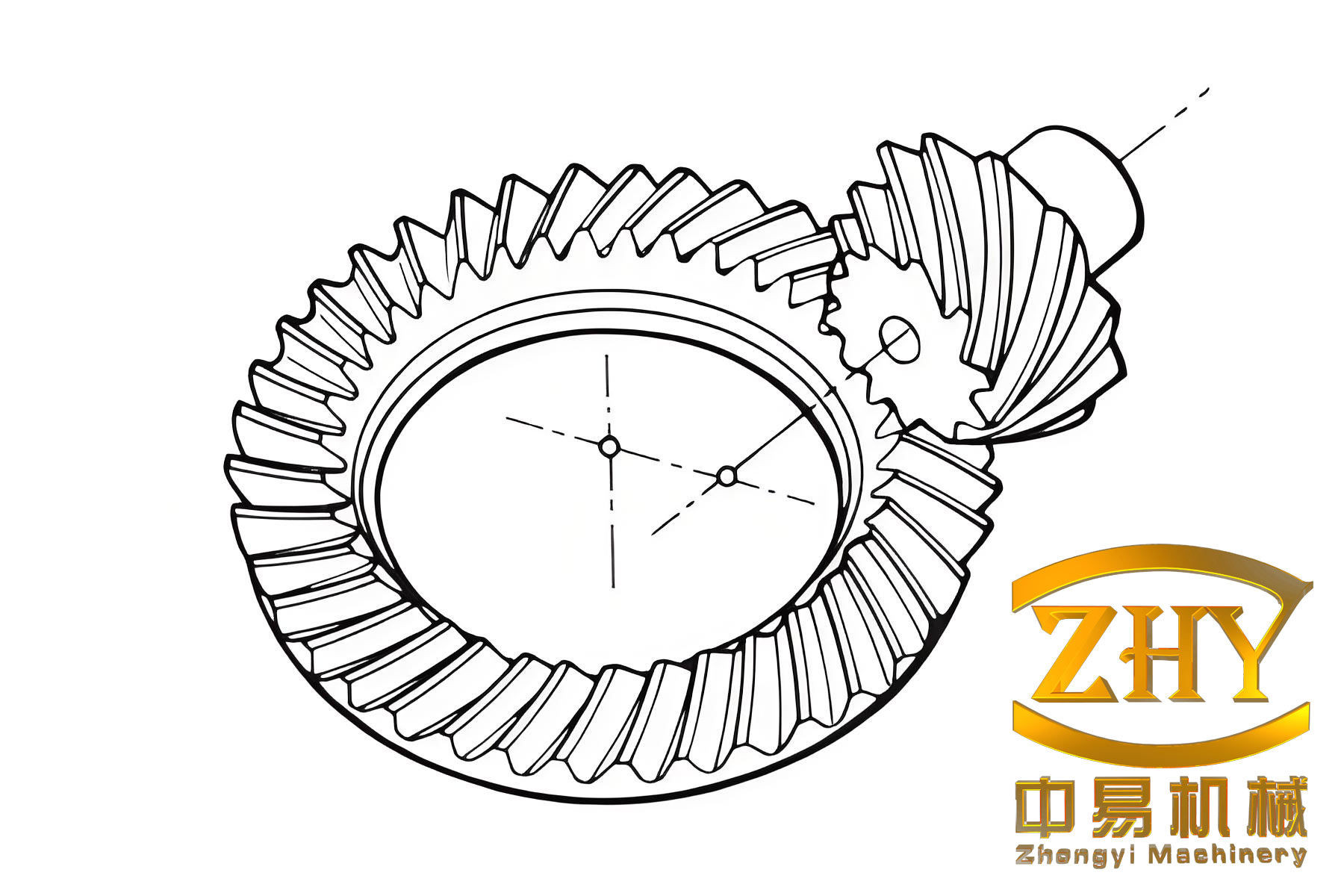
This study focuses on the calculation methodology for the sliding rate of high-reduction ratio hypoid bevel gears. We begin by proposing a novel iterative method for calculating the fundamental blank parameters of these gears. Subsequently, based on spatial gear meshing principles, we analyze the kinematic state of point contact and derive the general formula for sliding rate. Finally, we apply this general theory specifically to high-reduction ratio hypoid bevel gears, incorporating their unique design parameters to establish a dedicated sliding rate calculation model. This research aims to provide a new computational tool for the design of high-reduction ratio hypoid bevel gear blanks and establish a theoretical basis for their wear analysis and optimization.
A Novel Calculation Method for Hypoid Bevel Gear Blank Parameters
The design of hypoid bevel gears, especially high-reduction ratio variants, begins with determining the gear blank parameters. These parameters define the basic geometry of the gear before tooth cutting. We propose a new calculation method derived from the GLEASON hypoid gear calculation card. This method initiates the calculation from the gear (large wheel) parameters and iteratively solves for the corresponding pinion (small wheel) blank parameters, which is particularly suited for high reduction ratios.
The spatial location of the pitch point is key to defining the pitch cones of a hypoid bevel gear pair. Three independent parameters are required to define this point in space. In our method, we use the gear pitch radius $r_2$, the pinion spiral angle $\beta_1$, and the pinion shaft offset angle $\eta$. The following outlines the steps to determine these parameters and subsequently calculate the fundamental blank dimensions for both members of the hypoid bevel gear pair.
First, based on transmission requirements, the following are specified: shaft angle $\Sigma$, number of teeth for gear $Z_2$ and pinion $Z_1$, hand of spiral, and pinion offset distance $E$. The gear pitch diameter $d_2$ is selected based on load capacity requirements. The gear face width $b_2$ should not exceed $10 m_t$ or one-third of the outer cone distance of an equivalent spiral bevel gear, where $m_t$ is the transverse module. The gear pitch angle is initially approximated using the GLEASON recommended formula:
$$ \tan \delta’_2 = \frac{Z_2 \sin \Sigma}{1.2 (Z_1 + Z_2 \cos \Sigma)} $$
The mean gear pitch radius is then calculated as:
$$ r_2 = \frac{1}{2}(d_2 – b_2 \sin \delta’_2) $$
The gear shaft offset angle is determined by:
$$ \sin \varepsilon’_0 = \frac{E \sin \delta’_2}{r_2} $$
An initial value for the pinion spiral angle is chosen, typically $\beta_{20} \approx 35^\circ$. An initial lengthening factor $k’$ is introduced:
$$ k’ = \frac{1}{\cos \varepsilon’_0 – \tan \beta_{20} \sin \varepsilon’_0} $$
The initial pinion pitch radius is:
$$ r’_1 = k’ i_{12} r_2 $$
where $i_{12}=Z_1/Z_2$ is the gear ratio. The pinion shaft offset angle $\eta$ is found through an iterative process starting with:
$$ \tan \eta = \frac{E}{r_2 (\tan \delta’_2 \sin \Sigma + \cos \Sigma) + r’_1} $$
If $|\tan \eta| \le 0.01$, set $\tan \eta = \pm 0.011$ (sign same as Eq. (1)). Using this value, approximate values for the gear shaft offset angle $\varepsilon$, pinion pitch angle $\delta_1$, offset angle $\varepsilon’$, and pinion spiral angle $\beta_1$ are calculated:
$$
\begin{aligned}
\sin \varepsilon_1 &= (E – r’_1 \sin \eta) / r_2 \\
\tan \delta’_1 &= \frac{\sin \eta}{\tan \varepsilon_1 \sin \Sigma} – \cot \Sigma \cos \eta \\
\sin \varepsilon’_1 &= \frac{\sin \varepsilon_1 \sin \Sigma}{\cos \delta_1} \\
\cos \varepsilon_1 &= \sqrt{1 – \sin^2 \varepsilon’_1}
\end{aligned}
$$
The approximate gear spiral angle is:
$$ \tan \beta’_2 = \frac{k’ \cos \varepsilon’_1 – 1}{k’ \sin \varepsilon’_1} $$
Since $\beta’_2$ may not equal the desired $\beta_{20}$, the lengthening factor is corrected. The corrected factor is $ k = \frac{1}{\cos \varepsilon’_1 – \tan \beta_{20} \sin \varepsilon’_1} $. Comparing $k$ with $k’$ yields a new factor used to calculate an updated pinion pitch radius $ r_1 = k i_{12} r_2 $. The parameters $\varepsilon, \delta_1, \varepsilon’, \beta_1$ are then recalculated more accurately:
$$
\begin{aligned}
\sin \varepsilon &= \sin \varepsilon_1 – i_{12}(k – k’) \sin \eta \\
\tan \delta_1 &= \frac{\sin \eta}{\tan \varepsilon \sin \Sigma} – \cot \Sigma \cos \eta \\
\tan \beta_2 &= \frac{k \cos \varepsilon’ – 1}{k \sin \varepsilon’} \\
\beta_1 &= \beta_2 + \varepsilon’
\end{aligned}
$$
The final gear pitch angle is:
$$ \tan \delta_2 = \frac{\sin \varepsilon}{\tan \eta \sin \Sigma – \cos \varepsilon \cot \Sigma} $$
The gear pitch cone distance is $R_2 = r_2 / \sin \delta_2$. The pinion pitch cone distance is:
$$ R_1 = \frac{r’_1 + i_{12}(k – k’)r_2}{\sin \delta_1} $$
Thus, the final pinion mean pitch radius is $r_1 = R_1 \sin \delta_1$. The limit pressure angle $\alpha^*$ is calculated to check the tooth geometry:
$$ \tan \alpha^* = \frac{ -\tan \delta_1 \tan \delta_2 \cos \varepsilon’ \frac{R_1 \sin \beta_1 – R_2 \sin \beta_2}{R_1 \tan \delta_1 + R_2 \tan \delta_2} } {1} $$
Note: The full expression from the source is complex; this is a simplified representation for structure. The actual formula includes terms in both numerator and denominator. The key output is the limit pressure angle $\alpha^*$ used in subsequent iteration checks.
The limit curvature radius $r^*$ is given by:
$$ r^* = \frac{1}{\cos \alpha^*} \frac{ \tan \beta_1 – \tan \beta_2 }{ -\tan\alpha^* \left( \frac{\tan \beta_1}{R_1 \tan \delta_1} + \frac{\tan \beta_2}{R_2 \tan \delta_2} \right) + \left( \frac{1}{R_1 \cos\beta_1} – \frac{1}{R_2 \cos \beta_2} \right) } $$
An iterative check is performed: if $|1 – r_0 / r^*| < 0.01$, where $r_0$ is the nominal cutter radius, the iteration concludes. Otherwise, a new value for $\tan \eta$ is estimated (e.g., using a secant method) and the process from Eq. (1) repeats until convergence.
The following table summarizes the key steps in this iterative calculation method for hypoid bevel gear blanks:
| Step | Description | Key Equations/Output |
|---|---|---|
| 1 | Input Design Specifications | $\Sigma, Z_1, Z_2, E, d_2, b_2, \beta_{20}$ |
| 2 | Calculate Initial Gear Parameters | $\delta’_2, r_2, \varepsilon’_0$ |
| 3 | Initial Pinion Estimation | $k’, r’_1, \eta$ (initial) |
| 4 | First Approximation | $\varepsilon_1, \delta’_1, \varepsilon’_1, \beta’_2$ |
| 5 | Correct Lengthening Factor | $k, r_1$ |
| 6 | Recalculate Precise Angles | $\varepsilon, \delta_1, \varepsilon’, \beta_1, \beta_2$ |
| 7 | Final Gear Pitch Angle | $\delta_2, R_2, R_1$ |
| 8 | Check & Iterate | Calculate $\alpha^*, r^*$, check $|1 – r_0/r^*| < 0.01$ |
This method provides a systematic approach to determining the fundamental geometry of high-reduction ratio hypoid bevel gears, which serves as the essential input for the subsequent sliding rate analysis.
Kinematic Analysis of Spatial Gear Meshing and Sliding Rate
To understand and calculate the sliding rate in hypoid bevel gears, we must first establish the general kinematic principles for spatial gearing. Consider two gears in mesh, denoted as gear 1 and gear 2. We establish three coordinate systems: a fixed reference system $S(O; x, y, z)$, and two moving systems $S_1(O_1; x_1, y_1, z_1)$ and $S_2(O_2; x_2, y_2, z_2)$ rigidly attached to gear 1 and gear 2, respectively. The angular velocities are $\boldsymbol{\omega}^{(1)}$ and $\boldsymbol{\omega}^{(2)}$, and the translational velocities of the origins are $\boldsymbol{v}_0^{(1)}$ and $\boldsymbol{v}_0^{(2)}$.
For a point $M$ in space, let its position vectors be $\boldsymbol{r}^{(1)}$ in $S_1$ and $\boldsymbol{r}^{(2)}$ in $S_2$. The absolute position vector from $O$ to $M$ is $\boldsymbol{r}$. We have $\boldsymbol{r} = \boldsymbol{r}_0^{(1)} + \boldsymbol{r}^{(1)}$, where $\boldsymbol{r}_0^{(1)}$ is the vector from $O$ to $O_1$. Differentiating with respect to time and applying the relation for derivatives in rotating frames yields the velocity of $M$ as observed from the fixed system but attached to gear 1:
$$ \frac{d\boldsymbol{r}}{dt} = \frac{d_1\boldsymbol{r}^{(1)}}{dt} + \boldsymbol{\omega}^{(1)} \times \boldsymbol{r}^{(1)} + \boldsymbol{v}_0^{(1)} $$
Here, $\frac{d_1\boldsymbol{r}^{(1)}}{dt}$ represents the relative velocity of $M$ within system $S_1$. A similar expression holds for gear 2. By relating these two expressions for the velocity of the same point $M$, we obtain the fundamental differential relationship for the motion of a contact point:
$$ d_2\boldsymbol{r}^{(2)} = d_1\boldsymbol{r}^{(1)} + \boldsymbol{v}^{(12)} dt $$
where $\boldsymbol{v}^{(12)}$ is the relative sliding velocity of gear 1 with respect to gear 2 at point $M$.
Now, consider the point contact condition between two tooth surfaces $\Sigma^{(1)}$ and $\Sigma^{(2)}$. At an instant, they contact at point $M$. After an infinitesimal time $dt$, the surfaces move to new positions $\Sigma^{(1)\prime}$ and $\Sigma^{(2)\prime}$. The point $M$ moves along the path of contact to $M’$. The corresponding points on the moved surfaces are $M_1$ (on $\Sigma^{(1)\prime}$) and $M_2$ (on $\Sigma^{(2)\prime}$). The differential vectors $d_1\boldsymbol{r}^{(1)} = \overrightarrow{MM_1}$ and $d_2\boldsymbol{r}^{(2)} = \overrightarrow{MM_2}$ represent the motion of the contact point along each surface. In general, these vectors have different directions in the tangent plane at $M$. If we choose the direction of $d_1\boldsymbol{r}^{(1)}$ to coincide with $\boldsymbol{v}^{(12)}$, then $d_2\boldsymbol{r}^{(2)}$ will also be in the same direction, but their magnitudes will differ by $|\boldsymbol{v}^{(12)}| dt$. This difference in the distance traveled by the contact point along the two surfaces is the essence of sliding.
The sliding ratios $\sigma_1$ and $\sigma_2$ for surface 1 and surface 2, respectively, are defined based on these differential displacements:
$$
\begin{aligned}
\sigma_1 &= \frac{|d_1\boldsymbol{r}^{(1)}| – |d_2\boldsymbol{r}^{(2)}|}{|d_1\boldsymbol{r}^{(1)}|} = 1 – \frac{|d_2\boldsymbol{r}^{(2)}|}{|d_1\boldsymbol{r}^{(1)}|} \\
\sigma_2 &= \frac{|d_2\boldsymbol{r}^{(2)}| – |d_1\boldsymbol{r}^{(1)}|}{|d_2\boldsymbol{r}^{(2)}|} = 1 – \frac{|d_1\boldsymbol{r}^{(1)}|}{|d_2\boldsymbol{r}^{(2)}|}
\end{aligned}
$$
A general formula derived from spatial gearing theory for the sliding rates at a contact point is:
$$
\begin{aligned}
\sigma_1 &= -\frac{ (\boldsymbol{v}^{(12)}, \boldsymbol{\omega}^{(12)}, \boldsymbol{n}) + |\boldsymbol{v}^{(12)}|^2 \cdot k_v^{(1)} }{ \boldsymbol{n} \cdot \boldsymbol{q} } \\
\sigma_2 &= \frac{ (\boldsymbol{v}^{(12)}, \boldsymbol{\omega}^{(12)}, \boldsymbol{n}) + |\boldsymbol{v}^{(12)}|^2 \cdot k_v^{(1)} }{ \boldsymbol{n} \cdot \boldsymbol{q} + (\boldsymbol{v}^{(12)}, \boldsymbol{\omega}^{(12)}, \boldsymbol{n}) + |\boldsymbol{v}^{(12)}|^2 \cdot k_v^{(1)} }
\end{aligned}
$$
where:
- $\boldsymbol{n}$ is the common unit normal vector to both surfaces at the contact point $M$.
- $\boldsymbol{\omega}^{(12)} = \boldsymbol{\omega}^{(1)} – \boldsymbol{\omega}^{(2)}$ is the relative angular velocity vector.
- $k_v^{(1)}$ is the normal curvature of surface $\Sigma^{(1)}$ in the direction of $\boldsymbol{v}^{(12)}$.
- $(\boldsymbol{v}^{(12)}, \boldsymbol{\omega}^{(12)}, \boldsymbol{n})$ denotes the scalar triple product.
- $\boldsymbol{q}$ is a characteristic vector given by $\boldsymbol{q} = \boldsymbol{\omega}^{(1)} \times (\boldsymbol{\omega}^{(2)} \times \boldsymbol{r}^{(2)}) – \boldsymbol{\omega}^{(2)} \times (\boldsymbol{\omega}^{(1)} \times \boldsymbol{r}^{(1)})$.
This general framework forms the basis for deriving the specific sliding rate formula for hypoid bevel gears.
Derivation of Sliding Rate Formula for High-Reduction Ratio Hypoid Bevel Gears
We now apply the general spatial meshing theory to the specific case of high-reduction ratio hypoid bevel gears. We aim to express the sliding rate in terms of the gear blank design parameters calculated in Section 1. The analysis focuses on the pitch point $M$, which is a specific, significant point on the tooth surface.
Using the gear blank parameters ($\delta_1, \delta_2, \beta_1, \beta_2, R_1, R_2, \varepsilon’, r_1, r_2$), we establish a local coordinate system $(M; \boldsymbol{i}, \boldsymbol{j}, \boldsymbol{k})$ at the pitch point $M$. The vector $\boldsymbol{k}$ is perpendicular to the pitch plane (the plane tangent to both pitch cones at $M$). Vectors $\boldsymbol{i}$ and $\boldsymbol{j}$ lie in this pitch plane. The angular velocity vectors $\boldsymbol{\omega}^{(1)}$ and $\boldsymbol{\omega}^{(2)}$ are along their respective gear axes. The geometry leads to the following relations for the vectors from the pitch cone apexes to $M$:
$$
\begin{aligned}
\overrightarrow{O’M} &= -L_1 (\sin \beta_1 \boldsymbol{i} – \cos \beta_1 \boldsymbol{j}) = -R_1 \sin\delta_1 (\sin \beta_1 \boldsymbol{i} – \cos \beta_1 \boldsymbol{j}) \\
\overrightarrow{O”M} &= -L_2 (\sin \beta_2 \boldsymbol{i} – \cos \beta_2 \boldsymbol{j}) = -R_2 \sin\delta_2 (\sin \beta_2 \boldsymbol{i} – \cos \beta_2 \boldsymbol{j})
\end{aligned}
$$
where $L_1 = R_1 \sin\delta_1$ and $L_2 = R_2 \sin\delta_2$. Therefore, the angular velocities can be expressed as:
$$
\begin{aligned}
\boldsymbol{\omega}^{(1)} &= \omega_1 (\cos \delta_1 \sin \beta_1 \boldsymbol{i} – \cos \delta_1 \cos \beta_1 \boldsymbol{j} – \sin \delta_1 \boldsymbol{k}) \\
\boldsymbol{\omega}^{(2)} &= \omega_2 (-\cos \delta_2 \sin \beta_2 \boldsymbol{i} + \cos \delta_2 \cos \beta_2 \boldsymbol{j} – \sin \delta_2 \boldsymbol{k})
\end{aligned}
$$
The relative angular velocity is:
$$ \boldsymbol{\omega}^{(12)} = (\omega_1 \cos \delta_1 \sin \beta_1 + \omega_2 \cos \delta_2 \sin \beta_2)\boldsymbol{i} – (\omega_1 \cos \delta_1 \cos \beta_1 + \omega_2 \cos \delta_2 \cos \beta_2)\boldsymbol{j} + (-\omega_1 \sin \delta_1 + \omega_2 \sin \delta_2)\boldsymbol{k} $$
The velocities of point $M$ as a point on each gear body are:
$$
\begin{aligned}
\boldsymbol{v}^{(1)} &= \boldsymbol{\omega}^{(1)} \times \overrightarrow{O’M} = \omega_1 L_1 (\sin \delta_1 \cos \beta_1 \boldsymbol{i} + \sin \delta_1 \sin \beta_1 \boldsymbol{j}) \\
\boldsymbol{v}^{(2)} &= \boldsymbol{\omega}^{(2)} \times \overrightarrow{O”M} = \omega_2 L_2 (\sin \delta_2 \cos \beta_2 \boldsymbol{i} + \sin \delta_2 \sin \beta_2 \boldsymbol{j})
\end{aligned}
$$
The relative sliding velocity $\boldsymbol{v}^{(12)} = \boldsymbol{v}^{(1)} – \boldsymbol{v}^{(2)}$. At the pitch point, by definition, the components of $\boldsymbol{v}^{(1)}$ and $\boldsymbol{v}^{(2)}$ along the common tangent in the direction of motion (often aligned with $\boldsymbol{j}$) are equal, meaning their difference in the $\boldsymbol{i}$-direction is zero. This leads to the condition $\omega_1 L_1 \sin \delta_1 \cos \beta_1 = \omega_2 L_2 \sin \delta_2 \cos \beta_2$. Using this and the geometric relation $\sin \varepsilon’ = (\sin \beta_1 \cos \beta_2 – \cos \beta_1 \sin \beta_2)$, the magnitude of the relative sliding velocity simplifies to:
$$ |\boldsymbol{v}^{(12)}| = \omega_1 L_1 \sin \delta_1 \sin \varepsilon’ \cos \beta_2 $$
and its direction is along $\boldsymbol{j}$.
The unit normal vector $\boldsymbol{n}$ at the tooth surface point $M$ depends on the pressure angle $\alpha$. For a hypoid bevel gear, $\boldsymbol{n} = \pm \cos \alpha \boldsymbol{i} + \sin \alpha \boldsymbol{k}$, where the upper sign (+) typically applies to the gear concave side (pinion convex side), and the lower sign (-) applies to the gear convex side. When the pressure angle equals the limit pressure angle $\alpha_0$, the point $M$ is a limit point. The limit pressure angle is given by:
$$ \tan \alpha_0 = \pm \frac{ L_1 \sin \beta_1 – L_2 \sin \beta_2 }{ L_1 \tan \delta_1 + L_2 \tan \delta_2 } $$
with the corresponding limit normal vector $\boldsymbol{n}_0 = \pm \cos \alpha_0 \boldsymbol{i} + \sin \alpha_0 \boldsymbol{k}$. The general normal vector can be expressed in terms of $\boldsymbol{n}_0$ and $\boldsymbol{k}$:
$$ \boldsymbol{n} = \frac{\cos \alpha}{\cos \alpha_0} \boldsymbol{n}_0 + \frac{\sin(\alpha – \alpha_0)}{\cos \alpha_0} \boldsymbol{k} $$
We also compute the dot product $\boldsymbol{n} \cdot \boldsymbol{q}$ and the scalar triple product $(\boldsymbol{v}^{(12)}, \boldsymbol{\omega}^{(12)}, \boldsymbol{n})$, where $\boldsymbol{q}$ is the characteristic vector. After substantial algebraic manipulation using the gear blank parameter relations, these expressions simplify to forms involving the basic design parameters. Specifically:
$$ \boldsymbol{n} \cdot \boldsymbol{q} = \frac{\sin(\alpha – \alpha_0)}{\cos \alpha_0} \omega_1 \omega_2 \cos \varepsilon’ (L_2 \sin \delta_2 \cos \delta_1 + L_1 \sin \delta_1 \cos \delta_2) $$
The scalar triple product is given by the determinant:
$$ (\boldsymbol{v}^{(12)}, \boldsymbol{\omega}^{(12)}, \boldsymbol{n}) =
\begin{vmatrix}
0 & \omega_1 L_1 \sin \delta_1 \sin \beta_1 – \omega_2 L_2 \sin \delta_2 \sin \beta_2 & 0 \\
\omega_1 \cos \delta_1 \sin \beta_1 + \omega_2 \cos \delta_2 \sin \beta_2 & \omega_1 \cos \delta_1 \cos \beta_1 + \omega_2 \cos \delta_2 \cos \beta_2 & -\omega_1 \sin \delta_1 + \omega_2 \sin \delta_2 \\
\cos \alpha & 0 & \sin \alpha
\end{vmatrix}
$$
Finally, the normal curvature $k_v^{(1)}$ in the direction of $\boldsymbol{v}^{(12)}$ for the pinion tooth surface can be calculated using standard differential geometry formulas for gear surfaces, based on the machine-tool settings and gear blank parameters.
Substituting all these component expressions into the general sliding rate formulas yields the final calculation model for high-reduction ratio hypoid bevel gears. For the pinion surface (taking gear concave side as surface 1), the sliding rate $\sigma_1$ is:
$$
\sigma_1 = -\frac{
\begin{vmatrix}
0 & \omega_1 L_1 \sin \delta_1 \sin \beta_1 – \omega_2 L_2 \sin \delta_2 \sin \beta_2 & 0 \\
\omega_1 \cos \delta_1 \sin \beta_1 + \omega_2 \cos \delta_2 \sin \beta_2 & \omega_1 \cos \delta_1 \cos \beta_1 + \omega_2 \cos \delta_2 \cos \beta_2 & -\omega_1 \sin \delta_1 + \omega_2 \sin \delta_2 \\
\cos \alpha & 0 & \sin \alpha
\end{vmatrix}
+ (\omega_1 L_1 \sin \varepsilon’ \cos \beta_2)^2 \cdot k_v^{(1)}
}{
\frac{\sin(\alpha – \alpha_0)}{\cos \alpha_0} \omega_1 \omega_2 \cos \varepsilon’ (L_2 \sin \delta_2 \cos \delta_1 + L_1 \sin \delta_1 \cos \delta_2)
}
$$
The corresponding sliding rate $\sigma_2$ for the gear surface can be obtained analogously or from the relation $\sigma_2 = \frac{\sigma_1}{\sigma_1 – 1}$ derived from the definitions. This formula explicitly expresses the sliding rate at the pitch point as a function of the fundamental hypoid bevel gear design parameters: angular velocities ($\omega_1, \omega_2$), pitch cone angles ($\delta_1, \delta_2$), spiral angles ($\beta_1, \beta_2$), pitch cone distances ($L_1, L_2$ or $R_1, R_2$), offset angle ($\varepsilon’$), pressure angle ($\alpha$), limit pressure angle ($\alpha_0$), and surface normal curvature ($k_v^{(1)}$).
Example Calculation and Verification for Hypoid Bevel Gears
To demonstrate the application of the proposed blank parameter calculation method and the derived sliding rate formula, we consider two example pairs of high-reduction ratio hypoid bevel gears. The first pair has a gear ratio of 3:45, and the second has a ratio of 5:60. Using the iterative method described in Section 1, the basic design parameters for these hypoid bevel gear pairs are calculated and summarized in the table below.
| Parameter | Symbol | 3:45 Gear Pair | 5:60 Gear Pair | Unit |
|---|---|---|---|---|
| Gear Teeth | $Z_2$ | 45 | 60 | – |
| Pinion Teeth | $Z_1$ | 3 | 5 | – |
| Normal Module | $m_n$ | 1.067 | 1.360 | mm |
| Shaft Angle | $\Sigma$ | 90 | 90 | deg |
| Pinion Offset | $E$ | 10 | 14 | mm |
| Pressure Angle | $\alpha$ | 20 | 19 | deg |
| Gear Spiral Angle | $\beta_2$ | 39.00 | 55.15 | deg |
| Pinion Spiral Angle | $\beta_1$ | 67.10 | 31.12 | deg |
| Gear Pitch Angle | $\delta_2$ | 77.60 | 84.17 | deg |
| Pinion Pitch Angle | $\delta_1$ | 10.99 | 5.33 | deg |
| Gear Face Width | $b_2$ | 9.24 | 16.08 | mm |
| Gear Outer Diameter | $d_{a2}$ | 48.01 | 81.65 | mm |
| Pinion Outer Diameter | $d_{a1}$ | 10.41 | 14.10 | mm |
For the sliding rate calculation, we focus on the gear concave side and the pinion convex side. Substituting the parameters for each hypoid bevel gear pair into the derived formula, and assuming appropriate values for the normal curvature $k_v^{(1)}$ based on standard cutter radius and machine settings, we compute the absolute values of the sliding rates at the pitch point. The results are as follows:
| Gear Pair | Gear Sliding Rate $|\sigma_2|$ | Pinion Sliding Rate $|\sigma_1|$ |
|---|---|---|
| 3:45 | 1.2381 | 5.1999 |
| 5:60 | 0.6364 | 1.7505 |
The results clearly show that for both pairs of high-reduction ratio hypoid bevel gears, the absolute sliding rate of the pinion is significantly larger than that of the gear. This aligns perfectly with the practical observation in high-ratio hypoid bevel gear transmissions: the pinion experiences more severe wear and is often the life-limiting component due to its higher sliding velocities. The calculation confirms that the sliding rate at the pitch point is non-zero, indicating the presence of relative sliding even at this nominally pure-rolling point, which is a characteristic of hypoid and worm-type gears.
To verify the correctness of the derived formula, an independent check was performed for the 5:60 hypoid bevel gear pair. The spatial coordinates of the pitch point were determined based on the gear blank geometry. These coordinates, along with the kinematic data, were then substituted into a general algebraic expression for sliding rate derived from spatial kinematics (different from the parameter-explicit form derived here). The verification calculation yielded values of $|\sigma’_2| = 0.6176$ and $|\sigma’_1| = 1.7613$. The close agreement between these values ($0.6364$ vs. $0.6176$ for the gear, $1.7505$ vs. $1.7613$ for the pinion) and the consistent trend (pinion sliding rate > gear sliding rate) validate the accuracy and reliability of the sliding rate calculation model developed specifically for high-reduction ratio hypoid bevel gears.
Conclusion
This study presents a comprehensive methodology for analyzing the sliding rate in high-reduction ratio hypoid bevel gears. The primary contributions are threefold. First, a novel iterative calculation method for determining the fundamental blank parameters of hypoid bevel gears is proposed. This method starts from the gear parameters and derives the corresponding pinion parameters, providing a new and systematic design approach tailored for high reduction ratios.
Second, based on spatial gear meshing theory, a detailed kinematic analysis was conducted. This led to the derivation of a general sliding rate formula for point contact gear pairs. This general theory was then specifically applied to the geometry of hypoid bevel gears. By incorporating their unique design parameters—such as pitch cone angles, spiral angles, offset angle, and pressure angle—a specialized mathematical model was established. This model explicitly calculates the sliding rate at the pitch point as a function of these fundamental hypoid bevel gear design parameters.
Third, the practical application of the method was demonstrated through two numerical examples: hypoid bevel gear pairs with ratios of 3:45 and 5:60. The calculated sliding rates confirmed that the pinion experiences a significantly higher sliding rate than the gear, explaining its propensity for accelerated wear. The results were further verified through an independent calculation, confirming the model’s validity.
In summary, this research provides a new computational tool for the design phase of high-reduction ratio hypoid bevel gears by linking blank geometry directly to a key performance indicator (sliding rate). More importantly, it establishes a crucial theoretical foundation for subsequent wear analysis and optimization of these complex and highly stressed gear components. By understanding and quantifying the sliding behavior, designers can make informed choices about parameters, materials, and lubrication to enhance the durability and reliability of hypoid bevel gear drives in demanding applications like robotics and precision machinery.