
In modern mechanical systems, the trend toward higher speeds and heavier loads has made the vibration of gear transmission systems under elastohydrodynamic lubrication a critical research topic. The presence of an oil film alters both the meshing stiffness and the friction coefficient at the tooth surfaces, profoundly affecting the dynamic response of spur gears. As a result, a comprehensive understanding of how the lubricating film, the associated film stiffness, and the tooth friction jointly influence the vibration of spur gears is essential for accurate vibration prediction.
This study focuses on a spur gear pair, specifically addressing the prediction of vibration characteristics while considering elastohydrodynamic lubrication. The research integrates numerical modeling, experimental measurements, and deep learning techniques. In particular, the combined effect of the oil-film stiffness and the tooth-surface friction coefficient is investigated through a dynamic model of the spur gear system, and a BP neural network is proposed for efficient vibration prediction under parametric uncertainty. The following sections describe the theoretical foundations, simulation results, experimental validation, and the developed prediction model.
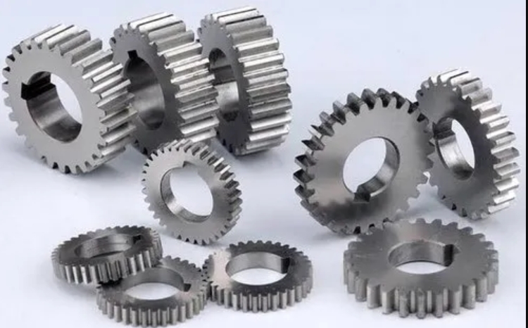
1 Introduction
Spur gears are widely used in automotive, aerospace, and industrial machinery because of their simple geometry, high efficiency, and compact design. However, their vibration behavior is strongly affected by the lubrication regime at the tooth contacts. Under normal operating conditions, the contact between tooth flanks is typically in the regime of elastohydrodynamic lubrication, where the lubricant film is very thin but capable of transmitting considerable pressure. The oil film alters the effective stiffness of the meshing teeth and produces a friction force that varies along the line of action. For a realistic prediction of spur gear vibration, both effects must be included simultaneously.
Earlier research frequently treated the oil-film stiffness and the tooth-surface friction coefficient independently. Many models focused on the influence of the oil film alone on the dynamic performance, while others studied friction-induced vibrations without considering the lubricating film. In practice, these two factors are coupled: the same operating conditions that change film thickness also change the friction coefficient. Therefore, an integrated approach is required to properly quantify the vibration response of spur gears under realistic lubrication conditions.
Another challenge arises from the random uncertainty of these parameters. The film thickness, and hence the film stiffness and the friction coefficient, fluctuate during a meshing cycle and vary with changing load and speed. Traditional dynamic models based on Newtonian mechanics often encounter difficulties when expecting accurate results for a wide range of operating conditions. In this context, machine learning techniques, specifically artificial neural networks, provide an alternative data-driven approach. These methods can learn complex nonlinear mappings from a set of input parameters to the vibration response, making them well suited for the prediction of spur gear dynamics under uncertainty.
The present work addresses these issues in a systematic manner. First, a line-contact elastohydrodynamic lubrication model is established to compute the oil-film pressure and thickness for spur gears. The oil-film stiffness is then derived and combined with the time-varying meshing stiffness to obtain a comprehensive meshing stiffness. Experimental measurements of torque losses are used to deduce the friction coefficients for various operating conditions. Second, a dynamic model of the spur gear pair is formulated, including the comprehensive meshing stiffness, the tooth-surface friction coefficient, the meshing damping, and the backlash. The influence of each parameter on the vibration response is analyzed. Third, experiments are carried out on a back-to-back gear test rig to validate the dynamic model. Finally, the uncertainties in the friction coefficient and the comprehensive stiffness are quantified, and a parallel BP neural network model is developed for the rapid prediction of spur gear vibration characteristics.
2 Oil-Film Lubrication and Meshing Stiffness
2.1 Governing equations of line-contact elastohydrodynamic lubrication
For a spur gear pair, the contact between the teeth at any instant can be modeled as a line contact between two equivalent cylinders with an equivalent radius of curvature. The Newtonian, isothermal, incompressible Reynolds equation in one dimension is:
$$
\frac{\partial}{\partial x}\left( \frac{\rho h^3}{12\eta}\frac{\partial p}{\partial x} \right) = u_e \frac{\partial (\rho h)}{\partial x} + \frac{\partial (\rho h)}{\partial t}
$$
where \(p\) is the oil-film pressure, \(h\) the film thickness, \(\rho\) the density, \(\eta\) the viscosity, \(x\) the coordinate along the entrainment direction, and \(u_e\) the entrainment velocity.
The film thickness equation for a line contact is expressed as:
$$
h(x,t) = h_0(t) + \frac{x^2}{2R} – \frac{2}{\pi E’} \int_{x_{in}}^{x_{out}} p(x’,t) \ln(x-x’)^2 dx’ + c
$$
with \(R\) the equivalent radius of curvature, \(E’\) the equivalent elastic modulus, \(h_0\) the rigid-body central film thickness, and \(c\) a constant determined from boundary conditions.
The viscosity-pressure relationship follows the Roelands equation:
$$
\eta = \eta_0 \exp\left\{ \left( \ln \eta_0 + 9.67 \right) \left[ \left( 1 + 5.1 \times 10^{-9} p \right)^{z_0} – 1 \right] \right\}
$$
where \(z_0\) is the Roelands pressure-viscosity index. The density-pressure relationship is given by the Dowson-Higginson equation:
$$
\rho = \rho_0 \left( 1 + \frac{0.6\times10^{-9} p}{1+1.7\times10^{-9} p} \right)
$$
The load balance equation is:
$$
\int_{x_{in}}^{x_{out}} p(x,t) dx = w(t)
$$
where \(w\) is the applied load per unit width. The above equations are solved numerically using the multigrid method, which is efficient for problems with strong nonlinearity and multiple length scales.
2.2 Oil film stiffness
The oil-film stiffness, which represents the resistance of the film to normal deformation, can be computed from the discrete pressure and thickness distributions. In this work, the normal stiffness of the oil film is calculated as:
$$
K_o = \frac{1}{\Delta H} \sum_{i=1}^{n} \frac{p_H \, n \, l \, R \, \Delta X \, P_i}{H_i}
$$
where \(P_i\) and \(H_i\) are the dimensionless pressure and film thickness at each grid point, \(\Delta X\) the grid spacing in the dimensionless domain, \(n\) the number of nodes, \(l\) the tooth width, and \(p_H\) the maximum Hertzian pressure.
2.3 Comprehensive meshing stiffness
The time-varying meshing stiffness of the spur gear pair is obtained using the Weber energy method. The tooth deformation is split into the bending, shear, and Hertzian contact components. The resulting meshing stiffness \(K_m(t)\) varies periodically as the number of contacting tooth pairs changes from one to two. Since the lubricating film acts as an additional compliance in series with the tooth stiffness, the comprehensive meshing stiffness \(K(t)\) is written as:
$$
K(t) = \frac{K_m(t) \cdot K_o(t)}{K_m(t) + K_o(t)}
$$
The parameters of the spur gear pair used in this study are listed in the following table.
Table 1: Gear parameters
| Parameter | Symbol | Pinion | Gear |
|---|---|---|---|
| Number of teeth | z | 24 | 16 |
| Module | m | 4.5 mm | |
| Pressure angle | α | 20° | |
| Addendum modification coefficient | x | -0.5 | 0.8532 |
| Face width | b | 20 mm | |
| Density | ρ | 7.8×10³ kg/m³ | |
| Bore diameter | d | 30 mm | |
2.4 Influence of operating conditions on comprehensive stiffness
Using the lubrication model and the stiffness calculation procedure, the variations of the oil-film stiffness and the comprehensive meshing stiffness along the line of action are analyzed. The results show that:
- As the torque increases from 50 N·m to 300 N·m at a constant speed of 1400 r/min, the oil-film thickness decreases, the film becomes harder to compress, and hence the oil-film stiffness increases. Consequently, the comprehensive meshing stiffness also increases.
- As the rotational speed increases from 400 r/min to 1800 r/min at a constant torque of 150 N·m, the entrainment velocity increases, causing the film thickness to grow. The oil film becomes softer, the film stiffness decreases, and the comprehensive meshing stiffness is reduced.
The typical time-varying comprehensive stiffness is compared with the conventional meshing stiffness in Table 2 for one representative operating condition.
Table 2: Comparison of meshing stiffness components
| Operating condition | Torque (N·m) | Speed (r/min) | Average oil-film stiffness (N/mm) | Average meshing stiffness (N/mm) | Average comprehensive stiffness (N/mm) |
|---|---|---|---|---|---|
| A | 150 | 800 | 2.86×10⁶ | 2.67×10⁵ | 2.48×10⁵ |
| B | 150 | 1400 | 1.62×10⁶ | 2.67×10⁵ | 2.32×10⁵ |
| C | 300 | 1400 | 3.12×10⁶ | 2.84×10⁵ | 2.69×10⁵ |
3 Measurement of Tooth-Surface Friction Coefficient
3.1 Experimental setup and power-loss method
The tooth-surface friction coefficient is difficult to measure directly. In this work, it is determined from the measured power losses in an FZG back-to-back gear test rig. The total power loss in the gearbox can be divided into load-independent losses (no-load losses) and load-dependent losses. The gear mesh power loss is obtained by subtracting the no-load losses, bearing losses, and seal losses from the total measured loss. The gear power loss is expressed as:
$$
P_{VZP} = P_{IN} \cdot U_V \cdot \mu
$$
where \(P_{IN}\) is the input power, \(U_V\) is a gear loss factor, and \(\mu\) is the friction coefficient. By rearranging this relationship, the friction coefficient can be computed from the measured gear mesh power loss:
$$
\mu = \frac{P_{VZP}}{P_{IN} \cdot U_V}
$$
The tests were performed with a LIQUI-MOLY 80W gear oil, maintaining the oil temperature between 35°C and 45°C. The test matrix included speeds of 400, 800, 1400, 1800, 3000, and 3500 r/min and torques of 5, 50, 150, and 300 N·m. The torque of 5 N·m was used to capture the no-load loss. The measured total torque loss is plotted against the operating parameters, and the resulting friction coefficient values are summarized below.
Table 3: Measured tooth-surface friction coefficients
| Speed (r/min) | Torque = 50 N·m | Torque = 150 N·m | Torque = 300 N·m |
|---|---|---|---|
| 400 | 0.0420 | 0.1505 | 0.2210 |
| 1400 | 0.0271 | 0.0814 | 0.1190 |
| 3500 | 0.0152 | 0.0554 | 0.0812 |
3.2 Discussion on friction coefficient behavior
The results indicate that the friction coefficient increases significantly with torque. For instance, at 1400 r/min, increasing the torque from 50 N·m to 300 N·m raises the friction coefficient from 0.0271 to 0.119, an increase of 339.1%. This occurs because a higher load reduces the film thickness, resulting in more direct asperity contacts. On the other hand, the friction coefficient decreases with increasing speed. At a torque of 150 N·m, raising the speed from 400 r/min to 3500 r/min reduces the coefficient from 0.1505 to 0.0554, a reduction of 63.2%. The higher speed increases the entrainment velocity and thus the film thickness, leading to better separation of the tooth surfaces and a lower friction coefficient.
4 Dynamic Model of Spur Gears
4.1 Lumped-parameter model
To investigate the coupled effects of the comprehensive meshing stiffness and the tooth-surface friction coefficient on the vibration of spur gears, a lumped-parameter model with six degrees of freedom is established. Each gear has two translational degrees of freedom (in the \(x\) and \(y\) directions) and one rotational degree of freedom. The differential equations are derived using Newton’s second law and Lagrange’s formulation. Let subscripts \(p\) and \(g\) denote the pinion and the gear, respectively. The equations are:
$$
\begin{cases}
m_p \ddot{x}_p + c_{px} \dot{x}_p + k_{px} x_p = F_f \sin\alpha + F_d \cos\alpha \\[4pt]
m_p \ddot{y}_p + c_{py} \dot{y}_p + k_{py} y_p = F_f \cos\alpha – F_d \sin\alpha \\[4pt]
I_p \ddot{\theta}_p + F_d r_{bp} – F_f R_p = T_p \\[4pt]
m_g \ddot{x}_g + c_{gx} \dot{x}_g + k_{gx} x_g = -F_f \sin\alpha – F_d \cos\alpha \\[4pt]
m_g \ddot{y}_g + c_{gy} \dot{y}_g + k_{gy} y_g = -F_f \cos\alpha + F_d \sin\alpha \\[4pt]
I_g \ddot{\theta}_g – F_d r_{bg} + F_f R_g = -T_g
\end{cases}
$$
where \(F_d\) is the dynamic meshing force, \(F_f\) is the friction force, \(R_p\) and \(R_g\) are the radii of curvature at the contact point, and \(r_{bp}\) and \(r_{bg}\) are the base radii.
The dynamic meshing force is:
$$
F_d(t) = K(t) f\!\left(\delta(t)\right) + c_m(t) \dot{\delta}(t)
$$
where \(K(t)\) is the comprehensive meshing stiffness, \(c_m(t)\) is the time-varying meshing damping, and \(\delta(t)\) is the relative displacement along the line of action:
$$
\delta(t) = \left( x_p – x_g \right)\sin\alpha + \left( y_p – y_g \right)\cos\alpha + r_{bp}\theta_p – r_{bg}\theta_g – e(t)
$$
The backlash nonlinearity is represented by the piecewise function:
$$
f(\delta) =
\begin{cases}
\delta – b_t, & \delta > b_t \\
0, & |\delta| \le b_t \\
\delta + b_t, & \delta < -b_t
\end{cases}
$$
where \(b_t\) is the half-backlash. The friction force on the tooth surface is given by:
$$
F_f(t) = \lambda \mu F_d(t)
$$
where \(\lambda\) defines the direction of the friction force, which changes at the pitch point.
4.2 Model parameters
The physical properties of the gears were obtained from a solid model. The mass and moment of inertia for the pinion and gear are listed in the following table.
Table 4: Gear inertia properties
| Parameter | Pinion | Gear |
|---|---|---|
| Mass (kg) | 1.17 | 0.64 |
| Moment of inertia (kg·m²) | 1.72×10⁻³ | 0.58×10⁻³ |
The time-varying meshing stiffness and damping are computed for each speed. Figure 3 in the original study shows the stiffness and damping as functions of time and frequency. The meshing frequency is defined as:
$$
f_m = \frac{n_p \cdot z_p}{60}
$$
where \(n_p\) is the pinion speed in revolutions per minute and \(z_p\) the number of teeth.
5 Vibration Characteristics of Spur Gears
5.1 Effect of comprehensive meshing stiffness
The dynamic model is solved numerically using a fourth-order Runge-Kutta method. To analyze the stability of the spur gear system with respect to the stiffness, bifurcation diagrams and the maximum Lyapunov exponent are used. The speed and torque are kept at 1400 r/min and 300 N·m, respectively, while the stiffness is varied over a realistic range.
The results show that the gear system remains in a single-period motion when the stiffness is relatively low, e.g., \(1.1\times10^5 \le K \le 1.73\times10^7\) N/mm. A sudden transition to quasi-periodic motion appears when the stiffness reaches \(1.74\times10^7\) N/mm, followed by a multi-periodic region. When the stiffness exceeds \(1.83\times10^7\) N/mm, chaotic behavior appears, and the system diverges when the stiffness grows beyond \(1.96\times10^7\) N/mm. These findings indicate that the oil-film stiffness contributes to the stability of the spur gear system by absorbing vibration energy and smoothing the meshing process.
The effect of the comprehensive stiffness on the vibration response is illustrated in Table 5. The amplitude of the steady-state vibration acceleration is reduced by 13.95% when the comprehensive stiffness is considered.
Table 5: Vibration acceleration amplitude with and without comprehensive stiffness
| Model | Steady amplitude (m/s²) | Peak at the fundamental meshing frequency (m/s²) |
|---|---|---|
| Without comprehensive stiffness | 4.30 | 1.41 |
| With comprehensive stiffness | 3.70 | 1.30 |
5.2 Effect of friction coefficient
Three representative friction coefficients are selected to study the influence of friction on the vibration of spur gears: \(\mu = 0.05\), \(\mu = 0.15\), and \(\mu = 0.25\). The simulations are performed at 1400 r/min and 300 N·m. The results, shown in the frequency spectra, indicate that the vibration accelerations at the fundamental meshing frequency and its harmonics increase as the friction coefficient increases. Table 6 gives the quantitative comparison.
Table 6: Effect of friction coefficient on vibration response
| Friction coefficient | Steady vibration amplitude (m/s²) | Peak at fundamental frequency (m/s²) | Increase compared to μ=0.05 |
|---|---|---|---|
| 0.05 | 1.50 | 1.40 | — |
| 0.15 | 1.90 | 1.90 | 26.7% |
| 0.25 | 2.40 | 2.30 | 60.0% |
5.3 Combined effect of friction and stiffness
In real operating conditions, the friction coefficient and the comprehensive stiffness change simultaneously with load and speed. To understand their interaction, the dynamic response is evaluated for different torques and speeds.
At a fixed speed of 1400 r/min, an increase in torque from 150 N·m to 300 N·m causes the comprehensive stiffness to increase, which alone would suppress vibration. However, the friction coefficient also rises due to a thinner oil film. The simulation results show that the overall vibration amplitude increases with torque, indicating that the friction effect outweighs the stiffness effect under these conditions. Table 7 summarizes the time-domain amplitudes and frequency-domain peaks.
Table 7: Vibration response at different torques (1400 r/min)
| Torque (N·m) | Steady amplitude (m/s²) | Peak at fundamental frequency (m/s²) |
|---|---|---|
| 150 | 3.6 | 1.50 |
| 200 | 4.4 | 1.71 |
| 300 | 5.6 | 2.53 |
At a fixed torque of 300 N·m, increasing the speed from 400 to 1400 r/min leads to a thicker oil film and a lower friction coefficient, which reduces the vibration. However, the comprehensive stiffness also decreases with speed, which would normally increase the vibration. The simulation indicates that the vibration amplitude is lower at 800 and 1400 r/min than at 400 r/min, demonstrating the dominant role of the friction reduction.
Table 8: Vibration response at different speeds (300 N·m)
| Speed (r/min) | Steady amplitude (m/s²) | Fundamental meshing frequency (Hz) |
|---|---|---|
| 400 | 4.7 | 160 |
| 800 | 4.0 | 320 |
| 1400 | 4.1 | 560 |
The phase portraits in the original study show that the system becomes more stable as the speed increases from 400 to 800 r/min, but becomes less stable again at higher speeds. This behavior is attributed to the competing effects of friction and stiffness: the friction-dominated regime improves stability up to 800 r/min, while the stiffness-dominated regime degrades stability beyond that speed.
6 Experimental Validation
6.1 Test rig and instrumentation
To validate the dynamic model, an FZG back-to-back gear test rig is used. The test rig consists of a test gearbox and a slave gearbox, connected by shafts. The gearbox is driven by a variable-speed motor, and a torque-loss sensor is installed between the motor and the slave gearbox. The vibration acceleration is measured with piezoelectric accelerometers mounted on the bearing housing of the test gearbox. A photoelectric tachometer records the shaft speed, and a thermocouple monitors the oil temperature.
Table 9: Sensor specification
| Instrument | Specification | Output |
|---|---|---|
| Accelerometer 1 | 10.169 mV/(m/s²) | Vibration acceleration |
| Accelerometer 2 | 10.209 mV/(m/s²) | Vibration acceleration |
| Photoelectric sensor | 10 mV per pulse | Rotational speed |
| Temperature sensor | PT100, 0.385 Ω/°C | Oil temperature |
6.2 Sweep-speed test
A sweep-speed test is performed with a constant torque of 20 N·m. The speed is continuously increased from 0 to 3000 r/min and then decreased back to 0 r/min. The measured vibration data are processed to generate three-dimensional spectral maps and order analyses. The results show that the vibration energy increases significantly with speed, especially in the high-frequency band of 3500–4500 Hz. The order analysis reveals a strong component at the third gear mesh order, which becomes dominant after 2400 r/min because the excitation frequency approaches a system natural frequency, causing resonance.
These results are consistent with the numerical simulations, thereby confirming that the dynamic model captures the speed-dependent vibration behavior of spur gears.
6.3 Constant-speed tests
Constant-speed tests are conducted at speeds of 400 r/min and 3500 r/min, and torques of 50 N·m and 150 N·m. The measured time-domain and frequency-domain responses are compared with the simulation results. For the condition of 400 r/min and 150 N·m, the root-mean-square value of the measured acceleration is 0.34 m/s², whereas the simulation gives 0.32 m/s², yielding an error of 6.3%. For 1400 r/min and 150 N·m, the measured and simulated values are 2.60 m/s² and 2.37 m/s², respectively, with an error of 9.7%. These errors are within acceptable limits, validating the accuracy of the proposed model.
A further comparison is made with a model that ignores both the comprehensive stiffness and the friction coefficient. For the same condition of 1400 r/min and 150 N·m, the error between the simplified model and the experiment is 19.3%, whereas the full model gives an error below 10%. This clearly demonstrates that including the elastohydrodynamic-lubrication effects is crucial for an accurate prediction of spur gear vibration.
7 Prediction of Vibration Characteristics Using BP Neural Networks
7.1 Uncertainty quantification
At each time step along the meshing cycle, the friction coefficient and the comprehensive stiffness are treated as random variables obeying truncated normal distributions satisfying the 3σ principle. The mean values are the calculated values from the previous sections, and the standard deviation is set to 0.83% of the mean, corresponding to a variation of ±2.5% over the 3σ range. The bootstrap method is used to compute 95% confidence intervals for these parameters at each time instant. An example interval is given in Table 10.
Table 10: Confidence intervals at selected time instants
| Time (s) | Friction coefficient interval | Comprehensive stiffness interval (N/mm) |
|---|---|---|
| 0.01 | [0.0987, 0.1031] | [178215.17, 178215.21] |
| 0.02 | [0.0987, 0.1035] | [263568.15, 263568.19] |
| 0.03 | [0.0988, 0.1034] | [159085.96, 159086.00] |
7.2 Dataset generation and preprocessing
The dynamic model described in Section 4 is used to generate a large dataset. The inputs are the comprehensive stiffness \(K\), the friction coefficient \(\mu\), the backlash function \(f(\delta)\), and the transmission error \(e(t)\). The outputs are the vibration acceleration \(a(t)\) and the dynamic meshing force \(F_d(t)\). The simulation is run at 1400 r/min and 150 N·m for a duration of 1 s. Data are sampled every 0.01 s, and the simulation is repeated 100 times, yielding 10,000 samples. In addition, a second dataset is created with data sampled along the line of action at very small time steps to capture the meshing-force variation over a single meshing period.
The dataset is preprocessed by removing missing values, detecting outliers using the z-score method, and applying a moving-average filter to reduce noise. After preprocessing, the data are normalized to the range [0, 1] using the min-max scaling method. The dataset is divided into training, validation, and test subsets with a ratio of 8:1:1.
Table 11 shows a few rows of the normalized dataset for the time-sampled case.
Table 11: Example of Normalized Training Data
| μ | K | f(δ) | e | a | F_d |
|---|---|---|---|---|---|
| 0.1053 | 0.2720 | 0.1456 | 0.6481 | 0.2449 | 0.2273 |
| 0.1182 | 0.5928 | 0.7978 | 0.7858 | 0.3401 | 0.6814 |
| 0.0806 | 0.0156 | 0.1855 | 0.2174 | 0.1716 | 0.2957 |
7.3 Architecture of the parallel BP neural network
A parallel connection of two BP neural networks (BPNN-PL) is designed for predicting the vibration acceleration and the dynamic meshing force simultaneously. The network for vibration acceleration has an input layer with four neurons, two hidden layers, and an output layer with one neuron. The network for dynamic meshing force has the same input configuration. The number of neurons in the hidden layers is determined by a trial-and-error procedure. The optimal numbers are found to be 11 for the acceleration network and 10 for the force network.
The activation function from the input layer to the first hidden layer is the tangent sigmoid function:
$$
\text{tansig}(x) = \frac{2}{1+e^{-2x}} – 1
$$
For the subsequent hidden layers and the output layer, the rectified linear unit function is used:
$$
\text{ReLU}(x) = \max(0, x)
$$
The Levenberg-Marquardt algorithm is used for training. The learning rate and the maximum number of epochs are set to 0.01 and 1200, respectively, after a grid search over a set of candidate values.
7.4 Performance evaluation
The prediction performance is evaluated using three metrics: the mean squared error (MSE), the mean absolute error (MAE), and the coefficient of determination \(R^2\). Their definitions are:
$$
\text{MSE} = \frac{1}{n} \sum_{i=1}^{n} \left( y_i – \hat{y}_i \right)^2
$$
$$
\text{MAE} = \frac{1}{n} \sum_{i=1}^{n} \left| y_i – \hat{y}_i \right|
$$
$$
R^2 = 1 – \frac{\sum_{i=1}^{n} \left( y_i – \hat{y}_i \right)^2}{\sum_{i=1}^{n} \left( y_i – \bar{y} \right)^2}
$$
The evaluation results for the test set are listed in Table 12.
Table 12: Performance of the BPNN-PL model
| Output | MSE | MAE | R² |
|---|---|---|---|
| Vibration acceleration | 0.020 | 0.109 | 0.996 |
| Dynamic meshing force (time-sampled) | 0.010 | 0.083 | 0.998 |
| Dynamic meshing force (line-of-action) | 0.008 | 0.061 | 0.998 |
The relative errors for the test samples are mostly less than 5% for all outputs. The average relative errors are found to be 2.26% for the vibration acceleration, 2.22% for the time-sampled meshing force, and 1.76% for the line-of-action meshing force. These results demonstrate the high accuracy of the trained model.
7.5 Comparison with experimental data
To assess the generalization capability of the BPNN-PL model, its predictions are compared with the experimental vibration accelerations measured at different operating conditions. Table 13 presents the root-mean-square values of the predicted and measured accelerations.
Table 13: Comparison of predicted and experimental vibration accelerations
| Speed (r/min) | Torque (N·m) | Predicted RMS (m/s²) | Experimental RMS (m/s²) | Error (%) |
|---|---|---|---|---|
| 1400 | 50 | 1.45 | 1.31 | 10.6 |
| 3500 | 50 | 12.65 | 11.81 | 7.1 |
| 1400 | 150 | 2.96 | 2.60 | 13.8 |
| 3500 | 150 | 46.84 | 42.97 | 9.1 |
The errors are around 10%, which is reasonable for engineering applications considering the idealized assumptions of the dynamic model and the measurement noise in the experimental setup. The predicted and measured acceleration waveforms share the same trend and similar dominant frequencies. Therefore, the proposed BPNN-PL model is considered reliable for the rapid prediction of the vibration characteristics of spur gears under elastohydrodynamic lubrication.
8 Conclusion
This work comprehensively investigated the vibration characteristics of spur gears under elastohydrodynamic lubrication and proposed an efficient prediction method using a parallel BP neural network. The main conclusions are as follows:
- The elastohydrodynamic lubrication model provided accurate predictions of the oil-film pressure and film thickness for spur gear contacts. Increasing torque increased the pressure and reduced the film thickness, while increasing speed increased the film thickness and reduced the oil-film stiffness.
- The comprehensive meshing stiffness, which combines the tooth stiffness with the oil-film stiffness, increased with torque and decreased with speed. The oil film was found to absorb vibration energy and improve the dynamic stability of the spur gear system.
- The tooth-surface friction coefficient increased substantially with torque, but decreased with speed. The friction coefficient had a more significant influence on the vibration response of spur gears than the comprehensive meshing stiffness in the investigated operating range.
- The dynamic model, which considered the comprehensive stiffness, friction, damping, and backlash, was validated by experiments. The root-mean-square errors between the simulated and measured vibration accelerations were below 10% for the tested conditions, demonstrating the model’s accuracy.
- A parallel BP neural network was developed to predict the vibration acceleration and dynamic meshing force. The model achieved high prediction accuracy with average relative errors lower than 5% on the test dataset. The comparison with experimental data showed errors of about 10%, confirming its generalization capability and practical utility.
These findings provide a solid theoretical basis for the vibration prediction and design optimization of spur gear drives under realistic lubrication conditions. The combination of physics-based modeling and data-driven prediction offers a promising approach for the efficient analysis of complex gear systems.