
In my work on hydraulic machinery, the pinion gear set is one of the most critical transmission components because it directly determines the reliability, safety, and operational stability of the entire drive system. When a pinion gear operates under complex working conditions, subtle changes in tooth contact, lubrication, and load distribution can gradually develop into wear or even broken tooth faults. These faults change the vibration signature of the pinion gear set, but traditional experience-based criteria and single-signal analysis methods often fail to provide stable and accurate identification. Therefore, I focused on effective representation of pinion gear running signals and constructed a fault diagnosis method based on vibration features and a support vector machine (SVM). By combining systematic implementation with experimental verification, I formed a complete engineering diagnosis workflow that improves both the accuracy and practical applicability of pinion gear fault identification.
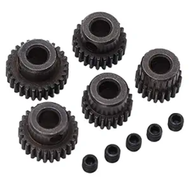
The core motivation of my study is that a hydraulic drive pinion gear set experiences time-varying loads, oil film fluctuations, and meshing impact forces. These factors make the vibration signal highly non-stationary. A normal pinion gear produces a relatively stable meshing frequency and low-level broadband noise. A worn pinion gear increases the energy of the meshing harmonics and introduces sidebands. A broken tooth pinion gear generates strong periodic impacts and transient components. If I can extract discriminative features from these signals and classify them with a robust nonlinear model, I can identify the health state of the pinion gear set with high confidence. This is the foundation of the method I present here.
Vibration Characteristics of Pinion Gear Sets
When a hydraulic mechanical drive pinion gear set becomes worn or loses a tooth, the energy level and impact characteristics of its vibration signal change noticeably. To quantitatively characterize the signal differences under different operating states, I selected the root mean square (RMS) value, crest factor, and kurtosis as fault feature parameters. These three parameters are widely used in rotating machinery diagnosis because they describe the signal from complementary perspectives: overall energy, impulsiveness, and peakness of distribution. For a pinion gear set, the RMS value reflects the general vibration severity, the crest factor indicates the strength of impact components caused by tooth damage, and kurtosis describes how sharply the signal deviates from a Gaussian distribution. In my experiments, these features showed clear separation among normal, slightly worn, and broken tooth pinion gear conditions.
The root mean square value of the vibration signal is used to reflect the overall energy level. I compute it as
$$ R = \sqrt{\frac{1}{n}\sum_{i=1}^{n} x_i^2} $$
where \(R\) is the RMS value of the vibration signal, \(n\) is the number of sampling points, and \(x_i\) is the vibration acceleration at the \(i\)-th sampling point. For a healthy pinion gear, the RMS value remains relatively low and stable. When the pinion gear surface wears, the RMS value increases because the friction and clearance-induced impacts raise the overall vibration energy. When a pinion gear tooth breaks, the RMS value rises further due to severe periodic impacts.
The crest factor is used to characterize the strength of impact components. I calculate it as
$$ C = \frac{\max |x_i|}{R} $$
where \(C\) is the crest factor and \(\max |x_i|\) is the maximum absolute amplitude of the vibration signal. A higher crest factor means that the signal contains stronger transient peaks relative to its average energy. For a pinion gear with a broken tooth, the crest factor becomes significantly larger than that of a normal pinion gear because each tooth loss event produces a sharp impulse.
Kurtosis is used to describe the peakedness of the signal distribution. I compute it as
$$ K = \frac{1}{n}\sum_{i=1}^{n}\left(\frac{x_i – \mu}{\sigma}\right)^4 $$
where \(K\) is kurtosis, \(\mu\) is the signal mean, and \(\sigma\) is the standard deviation. For a normal pinion gear, the vibration signal is closer to a Gaussian distribution, so kurtosis is around 3. For a worn pinion gear, the distribution becomes more peaked, and for a broken tooth pinion gear, the kurtosis increases sharply because of repeated impact events. Table 1 summarizes the statistical results of these feature parameters under different pinion gear operating states.
| Operating state | RMS (m·s-2) | Crest factor | Kurtosis |
|---|---|---|---|
| Normal pinion gear | 1.86 | 2.91 | 3.08 |
| Slight wear | 2.43 | 3.36 | 4.21 |
| Broken tooth | 3.97 | 4.82 | 7.35 |
From Table 1, I can observe that as the fault severity increases, all three feature parameters show an upward trend. This confirms that the selected features can effectively distinguish normal and faulty pinion gear states. The increase in RMS value indicates a rise in overall vibration energy. The increase in crest factor indicates stronger impact components. The increase in kurtosis indicates a more impulsive and non-Gaussian signal distribution. These trends are consistent with the physical behavior of a damaged pinion gear set under hydraulic drive conditions.
Diagnosis Flow Construction
Based on the operating characteristics and fault signal behavior of the pinion gear set, I constructed a complete fault diagnosis flow. First, I acquire vibration signals from the pinion gear set during operation using sensors. Second, I denoise and normalize the raw data to reduce the influence of environmental interference on feature calculation. Third, within a fixed time window, I extract RMS, crest factor, and kurtosis to form a feature vector that reflects differences in operating state. Fourth, I input the feature vector into an SVM diagnosis model and use its nonlinear classification capability to identify the pinion gear operating state. Finally, I determine the fault type according to the model output and achieve effective discrimination of the pinion gear running state. This flow maintains clear diagnostic logic while also ensuring engineering operability.
The diagnosis flow can be summarized in the following stages:
| Stage | Function | Output |
|---|---|---|
| Vibration signal acquisition | Collect pinion gear vibration data | Raw time-domain signal |
| Signal preprocessing | Denoise, normalize, and segment | Clean and standardized signal |
| Feature extraction | Compute RMS, crest factor, and kurtosis | Feature vector |
| SVM classification | Classify feature vector | Predicted state label |
| Fault decision | Stabilize and confirm diagnosis | Fault type and alarm |
This flow is designed for practical use on a hydraulic drive pinion gear set. It avoids relying on a single threshold and instead uses a learned decision boundary. The feature vector is low-dimensional, which reduces computational cost and makes real-time implementation feasible. At the same time, the SVM model can handle nonlinear relationships among features, which is important because the vibration behavior of a damaged pinion gear is not linearly separable in the original feature space.
SVM Diagnosis Model Establishment
I treat the pinion gear fault diagnosis problem as a supervised classification problem based on feature vectors. The input is a feature vector composed of RMS, crest factor, and kurtosis. The output is the corresponding operating state class. The SVM constructs an optimal classification hyperplane to effectively separate different fault states. The optimization objective function can be expressed as
$$ \min_{w,b,\xi} \frac{1}{2}\|w\|^2 + C\sum_{i=1}^{n}\xi_i $$
where \(w\) is the normal vector of the classification hyperplane, \(b\) is the bias term, \(\xi_i\) is the slack variable, and \(C\) is the penalty coefficient used to balance model complexity and misclassification cost. A larger \(C\) penalizes misclassification more strongly, while a smaller \(C\) allows more margin violations. In my implementation, I tuned \(C\) through cross-validation to achieve a good trade-off between generalization and training accuracy.
Considering the nonlinear relationships among pinion gear fault features, I selected the radial basis function (RBF) as the kernel function. The RBF kernel is defined as
$$ K(x_i, x_j) = \exp(-\gamma \|x_i – x_j\|^2) $$
where \(K(x_i, x_j)\) is the kernel function value used to measure the similarity between samples \(x_i\) and \(x_j\) in a high-dimensional feature space, \(x_i\) and \(x_j\) are the feature vectors corresponding to the \(i\)-th and \(j\)-th samples, \(\|\cdot\|\) is the Euclidean distance, and \(\gamma\) is the kernel parameter used to control the distribution scale after feature mapping. The RBF kernel is suitable for pinion gear diagnosis because it can map the original three-dimensional feature space into a higher-dimensional space where normal, worn, and broken tooth states become more separable.
Substituting the RBF kernel into the discriminant function, I obtain the final classification expression of the SVM as
$$ f(x) = \operatorname{sign}\left( \sum_{i=1}^{n} \alpha_i K(x_i, x) + b \right) $$
where \(f(x)\) is the discriminant function output, \(\operatorname{sign}(\cdot)\) is the sign function representing the predicted class label of the input sample, \(x\) is the feature vector of the sample to be classified, \(K(x_i, x)\) is the kernel function, and \(\alpha_i\) is the Lagrange multiplier. In my diagnosis model, the sign output is mapped to the three pinion gear states: normal, slight wear, and broken tooth. Because the problem is multi-class, I used a one-versus-one or one-versus-rest strategy during training and selected the class with the strongest decision value.
The SVM model has several advantages for pinion gear fault diagnosis. It works well with small samples, which is often the case in industrial fault diagnosis because collecting many faulty pinion gear samples is expensive. It has strong generalization ability due to margin maximization. It is also robust to high-dimensional feature spaces, although in my case the feature dimension is only three. The model training and prediction are fast enough for online monitoring of a hydraulic drive pinion gear set.
System Implementation
I implemented the pinion gear fault diagnosis system according to functional layers: a data acquisition layer, a data processing and feature analysis layer, and a diagnosis decision layer. The data acquisition layer obtains the raw signal from the pinion gear set through vibration sensors and completes signal conditioning and sampling to provide stable data input for subsequent analysis. The data processing and feature analysis layer preprocesses the acquired signal and calculates RMS, crest factor, and kurtosis to form a feature vector reflecting the pinion gear operating state. The diagnosis decision layer takes the feature vector as input, calls the SVM diagnosis model to complete operating state recognition, and outputs the corresponding fault category. This system structure can satisfy the real-time and reliability requirements of pinion gear fault diagnosis in engineering applications.
| Layer | Components | Main task |
|---|---|---|
| Data acquisition layer | Vibration sensor, signal conditioning, sampling | Collect raw pinion gear vibration signal |
| Data processing and feature analysis layer | Preprocessing, window segmentation, feature calculation | Generate feature vector for pinion gear state |
| Diagnosis decision layer | SVM model, fault classification, decision logic | Identify pinion gear fault type |
The layered design allows me to replace or upgrade individual modules without changing the entire system. For example, if a different sensor is used, only the acquisition layer needs adjustment. If a new feature is added, the feature analysis layer can be modified. If a more advanced classifier is developed, the diagnosis decision layer can be updated. This modularity is important for long-term maintenance and deployment on different hydraulic drive pinion gear sets.
Data Acquisition and Processing
The data acquisition and processing stage corresponds to the data acquisition layer and the front end of feature analysis. Its main task is to obtain stable and effective raw signals and provide reliable input for feature calculation. I continuously monitor the operating state of the pinion gear set through vibration sensors and acquire vibration signals that reflect changes in meshing state. To reduce the influence of environmental noise and random interference, I first denoise and amplitude-normalize the raw signal so that data under different working conditions are comparable. Then I segment the signal within a fixed time window to provide a consistent data basis for feature parameter calculation. This process ensures the accuracy and stability of feature extraction.
In my experiments, I set the sampling frequency to 5 kHz and the time window length to 1 s. Adjacent windows overlap by 50% to avoid missing transient events between windows. The overlapping segmentation is especially important for broken tooth pinion gear faults because the impact may occur near a window boundary. By overlapping, I increase the probability that the impact is fully captured in at least one window. I also apply a moving average or wavelet-based denoising method to suppress high-frequency noise while preserving the impact components that are relevant to pinion gear faults.
The normalization step maps the signal amplitude to a standard range, such as zero mean and unit variance. This prevents one feature from dominating the distance calculation in the SVM kernel. Without normalization, the RMS value, which has a larger numerical scale, could overshadow the crest factor and kurtosis. After normalization, all three features contribute more equally to the classification decision. I also remove outliers that are caused by sensor glitches rather than actual pinion gear faults. This step is important because a single large spike can distort kurtosis and crest factor values.
Diagnosis Model Training
Diagnosis model training corresponds to the diagnosis decision layer and is a key step for fault identification. I use the feature vectors output by the data processing and feature analysis layer as model inputs, label the samples according to the pinion gear operating state, and construct a training dataset and a test dataset. I use cross-validation to configure the penalty coefficient and kernel parameter combinations and select the parameter combination with the best classification performance as the final model settings. During training, I focus on the classification stability of the model for different fault states to avoid judgment errors caused by uneven sample distribution. After training, the SVM model forms a stable classification boundary.
For the pinion gear dataset, I used a grid search over \(C\) and \(\gamma\). The search range for \(C\) was from \(2^{-5}\) to \(2^{15}\), and the search range for \(\gamma\) was from \(2^{-15}\) to \(2^{5}\). I used five-fold cross-validation on the training set. The best parameter combination was selected based on the average validation accuracy. I also balanced the number of samples for normal, slight wear, and broken tooth pinion gear states. Although the original data collection may naturally contain more normal samples, I used resampling or class weighting to prevent the SVM from being biased toward the majority class. This is critical because a broken tooth pinion gear fault is rare in practice but has the highest safety impact.
After training, I evaluated the model on an independent test set. I also analyzed the confusion matrix to understand which fault types are most easily confused. In my experiments, the most common confusion was between normal and slight wear, because early wear may produce only a small increase in RMS and kurtosis. The broken tooth pinion gear state was more distinct because of its strong impacts. This analysis helped me refine the feature extraction and preprocessing steps.
Fault Decision Method
The fault decision method is located in the diagnosis decision layer. Its core task is to convert the SVM model output into a clear engineering diagnosis conclusion. After the model classifies the input feature vector, it outputs the corresponding operating state class, and I determine the current state of the pinion gear set according to the maximum discriminant result. When the diagnosis result remains consistent over consecutive decision cycles, I consider it a valid fault state and output the corresponding fault type information. If the result fluctuates, I maintain the current operating state and continue monitoring. This decision method ensures the reliability of the diagnosis result while reducing the influence of instantaneous interference on the decision, which satisfies the stability and operability requirements of engineering applications.
I implemented a persistence check with a window of \(m\) consecutive cycles. For example, if the SVM predicts the same fault class for three consecutive windows, the system confirms the fault. If the prediction alternates between normal and slight wear, the system keeps the normal state and raises a warning for further observation. This reduces false alarms caused by temporary load changes or oil pressure fluctuations in the hydraulic drive pinion gear set. The decision logic is simple but effective, and it can be adjusted according to the criticality of the pinion gear application. For a high-speed pinion gear set, a shorter confirmation window may be used to ensure rapid response. For a low-speed pinion gear set, a longer window may be used to improve stability.
Experimental Validation
The experimental object was a hydraulic mechanical drive pinion gear set. I used vibration sensors to collect operating signals. The sampling frequency was set to 5 kHz, the time window length was set to 1 s, and adjacent windows overlapped by 50%. The experimental conditions included three classes: normal, slight wear, and broken tooth fault. I collected 200 valid samples for each class. After unified denoising, normalization, and segmentation, I divided the data into a training set and a test set at a ratio of 7:3. The experiment was repeated under the same parameter configuration to ensure comparability and reliability of the results.
| Parameter | Value |
|---|---|
| Sampling frequency | 5 kHz |
| Time window length | 1 s |
| Window overlap | 50% |
| Classes | Normal, slight wear, broken tooth |
| Samples per class | 200 |
| Training/test split | 7:3 |
To objectively evaluate the recognition ability of the constructed SVM diagnosis model under different operating states, I selected three typical states: normal, slight wear, and broken tooth fault. The number of samples for each condition was kept the same. Under the same sampling frequency, time window, and preprocessing parameters, I completed feature extraction and model discrimination and calculated the diagnosis accuracy and other key indicators. The results are shown in Table 5. The model achieved a diagnosis accuracy of 96.5% for the normal state, 94.2% for slight wear, and 92.0% for the broken tooth fault. This indicates that the feature parameters and the SVM classification boundary have good discriminative ability. Compared with the normal condition, the diagnosis accuracy of the broken tooth fault decreased by 4.5 percentage points, mainly because the broken tooth introduced increased impact and non-stationary components, and the sample feature distributions overlapped to some extent.
| State type | Number of samples | Diagnosis accuracy (%) |
|---|---|---|
| Normal pinion gear | 200 | 96.5 |
| Slight wear | 200 | 94.2 |
| Broken tooth | 200 | 92.0 |
I also compared the proposed SVM-based method with a traditional feature threshold judgment method. Using the same vibration signal dataset, I completed feature extraction and fault identification under consistent sampling frequency, time window length, and preprocessing parameters to ensure the comparison was fair and comparable. The diagnosis results of the two methods are shown in Table 6. It can be seen that under normal, slight wear, and broken tooth states, the SVM diagnosis method achieved higher recognition accuracy than the traditional diagnosis method, and the improvement was most obvious under the broken tooth fault. The experimental results show that the SVM diagnosis method has stronger classification ability and adaptability under complex faults and can effectively improve the reliability of pinion gear fault diagnosis.
| State type | Traditional method accuracy (%) | SVM method accuracy (%) |
|---|---|---|
| Normal pinion gear | 91.0 | 96.5 |
| Slight wear | 87.5 | 94.2 |
| Broken tooth | 82.0 | 92.0 |
The comparative results confirm that the SVM method is more robust than fixed thresholds. A traditional threshold method requires manual selection of thresholds for RMS, crest factor, and kurtosis. These thresholds may work well for one pinion gear set but fail for another because of differences in load, speed, and structural dynamics. In contrast, the SVM learns the decision boundary from data, so it can adapt to different pinion gear operating conditions. The RBF kernel further allows nonlinear separation, which is important when the fault features overlap in the original space.
Discussion
The experimental results show that the proposed method can achieve high diagnosis accuracy for a hydraulic drive pinion gear set. The three features—RMS, crest factor, and kurtosis—provide complementary information. RMS captures the overall energy increase caused by wear and broken teeth. Crest factor captures the impulsiveness caused by tooth loss. Kurtosis captures the non-Gaussianity caused by impacts. When used together, they form a compact but informative feature vector. The SVM then finds a nonlinear boundary that separates the three states. The accuracy is above 92% for all three states, which meets the requirements of many engineering applications.
The slight reduction in accuracy for the broken tooth pinion gear state is understandable. A broken tooth generates strong impacts that may vary depending on the tooth engagement position, load level, and rotational speed. The vibration signal may also contain transient components that are not perfectly aligned with the fixed time window. In addition, the broken tooth state may share some features with severe wear, especially when the broken tooth occurs on a pinion gear that is already worn. To improve the accuracy further, I could use more advanced preprocessing such as order tracking, which synchronizes the signal with the pinion gear rotation and reduces speed fluctuations. I could also add more features such as sideband energy, envelope spectrum peaks, or wavelet packet energy. However, adding too many features may increase the risk of overfitting, so feature selection would be necessary.
From an engineering perspective, the method has several advantages. First, it uses only three features, so the computational load is low and real-time implementation is feasible. Second, the SVM model can be trained with a relatively small number of samples, which is practical because collecting broken tooth pinion gear data is difficult and expensive. Third, the decision logic with consecutive confirmation reduces false alarms, which is important in industrial environments where hydraulic drive pinion gear sets operate continuously. Fourth, the system is modular, so it can be integrated into an existing condition monitoring platform without major changes.
There are also limitations. The current study focuses on three states: normal, slight wear, and broken tooth. In real hydraulic machinery, a pinion gear may experience pitting, spalling, crack propagation, and misalignment. These faults may produce different vibration signatures. The SVM model would need to be retrained with additional classes to cover these conditions. The current method also assumes that the operating speed and load are relatively stable during the feature extraction window. If the speed changes rapidly, the frequency content of the vibration signal will shift, and the time-domain features may become less reliable. Future work could combine time-domain features with frequency-domain or time-frequency features to improve robustness under variable speed conditions.
Another direction for improvement is the use of multi-sensor data. In my current implementation, I used vibration sensors only. However, a hydraulic drive pinion gear set also produces pressure fluctuations, temperature changes, and acoustic emissions. Combining vibration with hydraulic pressure signals could provide additional information about the fault. For example, a broken tooth may cause a sudden pressure pulsation in the hydraulic circuit. A multi-source SVM model could fuse these signals and improve the diagnosis accuracy, especially for early-stage faults. This would require careful synchronization and feature-level or decision-level fusion.
Conclusion
I have presented an SVM-based fault diagnosis method for hydraulic mechanical drive pinion gear sets. The method analyzes the vibration characteristics of the pinion gear set under normal, wear, and broken tooth conditions and constructs an SVM diagnosis model using RMS, crest factor, and kurtosis as feature parameters. I also completed system implementation and experimental verification. The results show that the method has high recognition accuracy for different operating states, with diagnosis accuracy above 92% for all tested conditions. It can effectively distinguish typical fault types and has good engineering application value.
The main contributions of my work can be summarized as follows. I established a compact feature set that captures the energy, impulsiveness, and non-Gaussianity of pinion gear vibration signals. I designed a complete diagnosis flow that includes data acquisition, preprocessing, feature extraction, SVM classification, and fault decision. I implemented a layered system structure that supports real-time monitoring and modular upgrades. I validated the method experimentally and compared it with a traditional threshold method. The SVM method consistently outperformed the traditional method, especially for the broken tooth pinion gear fault.
For future work, I plan to expand the fault classes to include pitting, spalling, and misalignment. I also plan to incorporate speed normalization and order tracking to handle variable speed conditions. In addition, I will explore multi-sensor fusion to combine vibration with hydraulic pressure and temperature signals. These improvements should further enhance the adaptability and accuracy of the method in real-world hydraulic drive pinion gear applications. Overall, the proposed approach provides a practical and effective solution for pinion gear fault diagnosis and contributes to the safe and reliable operation of hydraulic mechanical transmission systems.