
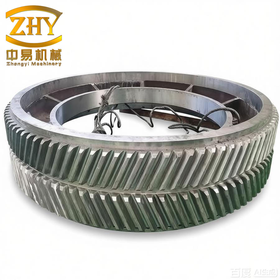
In the field of high-speed and heavy-duty power transmission, the herringbone gear is widely recognized because it combines the high load-carrying capacity of helical gears with a balanced axial thrust arrangement. A herringbone gear is manufactured by mounting two helical gear sections with opposite hands on the same gear blank. Ideally, these two sections are exactly symmetric with respect to a central plane, which is usually called the symmetry mid-plane. In reality, however, the manufacturing process cannot produce perfect symmetry. The resulting asymmetry of the herringbone gear causes non-uniform load distribution between the two halves, and often produces an unbalanced axial force. This axial force becomes particularly harmful in aviation transmissions, where high speed and high torque amplify the effect of any asymmetry. Therefore, it is important to characterize, measure and evaluate the symmetry deviation of the herringbone gear in a systematic way.
At present, the evaluation and inspection of herringbone gear symmetry deviation still lack a unified standard. Many existing concepts describe only one aspect of the asymmetry, e.g. a phase difference at a particular location, and therefore do not give a complete description of the actual tooth flank deviation. In response to this problem, I have studied the characterization of herringbone gear symmetry deviation, proposed a decomposition of the symmetry deviation into distance and angular components, designed a measurement method based on a coordinate measuring machine, implemented data-processing programs, and verified the method through experiments. In this paper I discuss all of these aspects and also investigate the influence of symmetry deviation on the meshing behavior of the herringbone gear by using finite element contact analysis.
1 Background and Problem Statement
The herringbone gear is a special cylindrical gear. It can be considered as two helical gears of opposite hand mounted coaxially. This configuration cancels the axial thrust produced by each helical half, and therefore allows a larger helix angle than an ordinary helical gear. The larger helix angle increases the contact ratio and the load capacity. Because of these advantages, the herringbone gear is often used in marine propulsion, aerospace transmissions, and other high-speed heavy-duty applications.
However, the production of a herringbone gear is more difficult than that of a spur or helical gear. The two helices must be machined separately, and any error in the relative angular position, radial position, helix angle, or tooth profile orientation of the two halves will create an undesirable symmetry deviation. The symmetry deviation of the herringbone gear has a direct influence on the contact pattern. If the load is concentrated on one side of the gear, the tooth surface stress increases, wear accelerates, and the risk of tooth breakage becomes higher. Moreover, the residual axial force caused by the asymmetry becomes an additional excitation source, leading to axial vibration and noise. In a high-speed aviation gearbox, this vibration can be extremely unfavorable to the gear system reliability.
Nevertheless, the measurement and evaluation of herringbone gear symmetry deviation are not sufficiently mature. Some methods use the intersection of extended helix lines with a central plane to define an alignment error. Other methods define a symmetry error by comparing corresponding points on opposite helical flanks. These definitions are useful, but they do not completely describe the three-dimensional geometric asymmetry of the herringbone gear. For this reason, I have attempted to establish a more complete representation of the symmetry deviation. I believe that a proper representation should include both distance deviation and angular deviation, and it should be expressed in the directions of the tooth profile and the helix.
2 Characterization of Herringbone Gear Symmetry Deviation
2.1 Transformation of the symmetry problem
The ideal herringbone gear is symmetric about its central plane. If one helical half is mirrored about the symmetry mid-plane, it should coincide exactly with the opposite helical half. In the actual herringbone gear, manufacturing errors make the mirrored tooth flank different from the opposite tooth flank. I therefore converted the symmetry deviation problem into a comparison of two tooth flanks. One flank is treated as the reference surface; the mirrored flank is treated as the measured surface. The difference between these two surfaces is exactly the herringbone gear symmetry deviation.
Using gear metrology theory, I considered the possible relative positions of two tooth flanks. The first possibility is a pure translation, producing a distance deviation. The second possibility is a rotation about an axis in the gear radial direction, which changes the helix angle. The third possibility is a rotation about a direction related to the tooth profile, which changes the profile orientation. In practice, the actual asymmetry is a combination of these three elementary states.
2.2 Basic gear errors used for the representation
Gear tooth flank errors are usually divided into tooth profile deviations and helix deviations. The tooth profile deviation describes how the actual tooth profile departs from an ideal involute. The helix deviation describes how the actual helix line departs from an ideal helix on a reference cylinder. Let me denote the tooth profile total deviation as \(F_\alpha\), the profile shape deviation as \(f_{f\alpha}\), and the profile slope deviation as \(f_{H\alpha}\). Similarly, the helix total deviation is denoted by \(F_\beta\), the helix shape deviation by \(f_{f\beta}\), and the helix slope deviation by \(f_{H\beta}\). Table 1 summarizes these basic error items.
| Error item | Symbol | Interpretation |
|---|---|---|
| Tooth profile total deviation | \(F_\alpha\) | Distance between two design profile lines that enclose the actual profile trace |
| Tooth profile shape deviation | \(f_{f\alpha}\) | Distance between two curves parallel to the mean profile enclosing the actual profile trace |
| Tooth profile slope deviation | \(f_{H\alpha}\) | Distance between two design profile lines intersecting the mean profile at the end points |
| Helix total deviation | \(F_\beta\) | Distance between two design helix lines that enclose the actual helix trace |
| Helix shape deviation | \(f_{f\beta}\) | Distance between two curves parallel to the mean helix enclosing the actual helix trace |
| Helix slope deviation | \(f_{H\beta}\) | Distance between two design helix lines intersecting the mean helix at the end points |
These basic gear errors show that tooth flank deviations cannot be described by a single distance only. It is necessary to separate a distance component and an angular component. Therefore, for the herringbone gear, I decomposed the symmetry deviation into four components:
- circumferential distance deviation \(L_s\);
- radial distance deviation \(L_R\);
- helix angular deviation \(L_\alpha\);
- tooth profile angular deviation \(L_\beta\).
These four components together characterize the symmetry state of the herringbone gear. Table 2 gives the calculation formulas used in my method.
| Symmetry deviation component | Symbol | Calculation formula |
|---|---|---|
| Radial distance deviation | \(L_R\) | \(L_R = R_1 – R_2\) |
| Circumferential distance deviation | \(L_s\) | \(L_s = r_\mathrm{ref}\,\Delta\varphi\) |
| Helix angular deviation | \(L_\alpha\) | \(L_\alpha = \dfrac{B\,\Delta\alpha}{\sin\beta}\) |
| Tooth profile angular deviation | \(L_\beta\) | \(L_\beta = \max(r_{k1}, r_{k2})\,|\theta_{k1}-\theta_{k2}|\) |
The helix angular deviation \(L_\alpha\) is converted from the difference between the helix angles of the two opposite herringbone gear flanks, while \(L_\beta\) is converted from the angular difference of the two mean tooth profile lines. In the formulas, \(B\) is the axial evaluation length, \(\beta\) is the nominal helix angle, and \(r_{k1}\) and \(r_{k2}\) are the radial coordinates of the common evaluation end of the two profile lines.
2.3 Mean helix and symmetric mid-plane intersection
To obtain the distance components, I first fit the measured helix points of each half into a mean helix line. I then extend the mean helix lines until they intersect the symmetry mid-plane. Because of the asymmetry, the two intersection points are not coincident. The two intersection points are denoted by \(A_1(x_1,y_1,z_1)\) and \(A_2(x_2,y_2,z_2)\). Their polar coordinates are:
\[
R_1=\sqrt{x_1^2+y_1^2},\qquad R_2=\sqrt{x_2^2+y_2^2}
\]
and their angular positions are:
\[
\varphi_1=\arctan\frac{y_1}{x_1},\qquad \varphi_2=\arctan\frac{y_2}{x_2}
\]
The radial distance deviation is then obtained directly:
\[
L_R=R_1-R_2
\]
The angular difference is:
\[
\Delta\varphi=\varphi_1-\varphi_2
\]
which is converted into a circumferential distance at the reference radius \(r_\mathrm{ref}\):
\[
L_s=r_\mathrm{ref}\,\Delta\varphi
\]
In my measurement, the reference radius was taken as the pitch cylinder radius. This choice is convenient because the helix lines are measured on the design pitch cylinder.
2.4 Angular components
The helix angular deviation of the herringbone gear is obtained from the mean helix lines of the two helical halves. Let the helix angles of the first and second halves be \(\alpha_1\) and \(\alpha_2\). Then:
\[
\Delta\alpha=\alpha_1-\alpha_2
\]
To express this angular difference as a linear deviation, I used the evaluated axial width \(B\) and the nominal helix angle \(\beta\):
\[
L_\alpha=\frac{B\,\Delta\alpha}{\sin\beta}
\]
This linearized value is comparable with the helix slope deviation defined in gear standards.
For the tooth profile angular deviation, I used the mean tooth profile lines fitted from the measured profile points of the opposite flanks. The two mean profile lines are first translated so that their involute starting points coincide. Then, at the common evaluation radius \(r_k\), the polar angle difference \(\theta_{k1}-\theta_{k2}\) is multiplied by the maximum radius in order to obtain a length value:
\[
L_\beta=\max(r_{k1},r_{k2})\,|\theta_{k1}-\theta_{k2}|
\]
This component is sensitive to the orientation of the whole profile, not merely to its position. Thus, the herringbone gear symmetry deviation cannot be represented by a single scalar. The four components defined above provide a more complete description.
3 Measurement Method and Program Design
3.1 Comparison of coordinate measuring strategies
The tooth flank of a gear can be measured using a coordinate measuring machine in three main ways: point measurement, feature-line measurement, and full-surface measurement.
In point measurement, one or several discrete points are extracted on each tooth flank. This method is efficient but it cannot reveal the orientation of the tooth flank. The measurement result strongly depends on the exact positions of the selected points, and it is difficult to reproduce the same point in repeated measurements. For this reason, point measurement is not sufficient for the evaluation of herringbone gear symmetry deviation.
Full-surface measurement provides the largest amount of information, but it is time-consuming. Moreover, if the definition of symmetry deviation is not fully established, a full point cloud is not directly useful.
Feature-line measurement is a compromise between efficiency and information content. I selected the helix line and the tooth profile line as the two characteristic lines. The helix line is measured on the reference cylinder and the tooth profile line is measured near the middle of the face width. This method provides enough points to determine both distance and angular deviations of the herringbone gear.
3.2 Helix line point extraction
For the helix line, the coordinate measuring machine moves a probe along the intersection curve between the tooth flank and the pitch cylinder. The probe records a series of points \(P_i\) with cylindrical coordinates \((r_p,\theta_i,z_i)\). The axial interval between adjacent points is set to \(\Delta Z\). For an ideal helix, the expected circumferential arc length between two adjacent points is:
\[
\omega_{\mathrm{th},i}=\Delta Z\,\tan\beta
\]
The actual arc length is obtained from the measured angular increment:
\[
\omega_i=r_p\,\Delta\theta_i
\]
where:
\[
\Delta\theta_i=\theta_{i+1}-\theta_i
\]
The helix deviation at each point is evaluated in a plane normal to the tooth flank:
\[
\Delta f_{\beta i}=\left(\omega_i-\omega_{\mathrm{th},i}\right)\cos\beta
\]
By applying this calculation to all measured points, I obtained the helix total deviation and the helix slope deviation for each half of the herringbone gear.
3.3 Tooth profile line point extraction
For the tooth profile line, the probe scans the involute profile at a fixed axial position. The most common scanning approach is to define a series of points on the involute with equal increments of the roll angle, but I also considered equal radial increment and equal involute arc length. Table 3 gives a summary of these strategies.
| Strategy | Sampling rule | Advantage | Disadvantage |
|---|---|---|---|
| Equal polar angle interval | Constant increment of \(\theta\) | Easy on rotary table | Unequal density in profile direction |
| Equal radial increment | Constant increment of \(r_k\) | Convenient for radial comparison | Not directly based on involute generation |
| Equal involute arc length | Constant increment of ideal involute length | Directly reflects involute quality | More complicated evaluation |
In my measurement program, I used the rectangular coordinate scanning mode of the coordinate measuring machine. After the raw point coordinates are obtained, the actual involute is constructed by least-squares fitting. The mean profile line is then compared with the theoretical involute.
The involute equations used in my program are:
\[
r_k=\frac{r_b}{\cos\alpha_k}
\]
\[
\theta_k=\mathrm{inv}\,\alpha_k=\tan\alpha_k-\alpha_k
\]
where \(r_b\) is the base radius and \(\alpha_k\) is the pressure angle at the evaluated point.
3.4 Reference coordinates and symmetry mid-plane
Because the symmetry mid-plane is a virtual plane, its position must be established before the measurement. In my method, the axis of rotation of the herringbone gear is used as the \(Z\)-axis of the measuring coordinate system. The symmetry mid-plane is then set as the \(XY\)-plane.
If the herringbone gear is machined with two end faces that are generated in the same setup, the mid-plane is located at the middle of the total face width. I measured both end faces with the probe and used their mid-plane as the symmetry mid-plane.
If the gear is made together with its shaft, as in the example I measured, the cylindrical shaft surfaces are used to establish the \(Z\)-axis, and the side faces of the shaft bosses are used to locate the symmetry mid-plane. The measurement procedure is as follows:
- Calibrate the probe and verify the coordinate measuring machine;
- Measure a cylindrical datum surface and define the \(Z\)-axis;
- Measure two reference planes and locate the symmetry mid-plane;
- Set the gear parameters in the gear measurement module;
- Select the target tooth gap and the target tooth flanks;
- Scan the helix lines and profile lines on both helical halves;
- Export the raw measurement data.
3.5 Data processing program
I wrote the data-processing program in MATLAB. The program reads the point coordinates collected by the coordinate measuring machine, converts the Cartesian coordinates into polar coordinates, fits the mean helix lines and mean profile lines, and finally calculates the four symmetry deviation components defined in Section 2.
The core fitting procedure for a measured helix line uses the following relation:
\[
\begin{cases}
x = r\cos\theta\\
y = r\sin\theta\\
z = c\,\theta + d
\end{cases}
\]
where \(r\) is the known reference radius, \(c\) and \(d\) are fitted parameters. The fitted value of \(c\) gives the actual helix angle. For the tooth profile line, I fitted an involute equation in the form:
\[
\sqrt{x^2+y^2}=\frac{r_b}{\cos\left(\theta-\theta_0\right)}
\]
where \(\theta_0\) is the initial roll angle of the fitted involute. This angle is useful for determining the tooth profile angular deviation \(L_\beta\).
The program also calculates the traditional tooth profile deviations and helix deviations. This is important because it allows me to compare my results with the results from the commercial gear measurement software installed on the coordinate measuring machine. The comparison validates the correctness of my data-processing program.
4 Measurement Experiment and Data Analysis
4.1 Measured herringbone gear parameters
I applied the proposed method to an aviation herringbone gear. The two helical halves have identical design parameters except for the hand of helix. Table 4 lists the main parameters of the measured herringbone gear.
| Parameter | Symbol | Value |
|---|---|---|
| Number of teeth | \(z\) | 27 |
| Normal module | \(m_n\) | 3.8788 mm |
| Normal pressure angle | \(\alpha_n\) | 22.5° |
| Helix angle | \(\beta\) | 30° |
| Tip diameter | \(d_a\) | 130.62 mm |
| Root diameter | \(d_f\) | 108.51 mm |
| Face width | \(b\) | 47 mm |
4.2 Coordinate measuring machine and probe
The measurement was carried out on a bridge-type coordinate measuring machine. Its main specifications are shown in Table 5.
| Specification | Value |
|---|---|
| X-axis travel | 800 mm |
| Y-axis travel | 1000 mm |
| Z-axis travel | 600 mm |
| Maximum workpiece weight | 500 kg |
| Length measurement error | \(3.0 + L/300\) μm |
| Scale resolution | 0.078 μm |
| Temperature | 20 ± 2 °C |
I used a ruby ball probe with a diameter of 1.0 mm. The small probe diameter was selected so that the probe could reach the narrow tooth spaces without interference. Before the measurement, the probe was calibrated with a reference sphere, and the machine was checked with gauge blocks. The calibration showed that the measuring error was within the permitted limit in all tested directions.
4.3 Helix line measurement results
I selected three groups of tooth gaps for the experiment. In each group, I measured one helix line on the left-hand flank and the corresponding helix line on the opposite right-hand flank. The measured points were imported into MATLAB and visualized together with the pitch cylinder and the symmetry mid-plane. The two mean helix lines were fitted and extended to the mid-plane.
For the first group, the average distance from the measured points to the fitted mean helix line was about 6.8 μm on the left-hand half and 4.0 μm on the right-hand half. The maximum distances were 16.8 μm and 20.5 μm respectively. These values show that the actual tooth flank is not perfectly helical and that the measured points scatter around the mean helix.
By comparing the two intersection points with the symmetry mid-plane, I obtained the symmetry deviation components. Table 6 lists the symmetry deviation results for the three groups.
| Group | \(L_s\) (μm) | \(L_R\) (μm) | \(L_\alpha\) (μm) | \(L_\beta\) (μm) |
|---|---|---|---|---|
| Group 1 | 15.3 | 10.2 | 5.3 | 6.3 |
| Group 2 | 13.6 | 8.5 | 6.5 | 5.9 |
| Group 3 | 17.8 | 11.7 | 7.2 | 8.4 |
The design drawing of this herringbone gear required the alignment error to be smaller than 20 μm. The largest circumferential distance deviation that I obtained was 17.8 μm, so this gear satisfies the drawing requirement. However, the measured profile angular deviation and helix angular deviation are also important because they influence the load distribution even when the circumferential deviation is below the drawing limit.
4.4 Tooth profile line measurement results
I also measured the tooth profile lines at the middle of the face width. The measured points were compared with the theoretical involute generated from the base circle. For the left-hand flank of the first group, the measured profile deviation was \(F_\alpha=10.8\) μm, the profile slope deviation was \(f_{H\alpha}=6.8\) μm, and the profile shape deviation was \(f_{f\alpha}=10.9\) μm. For the corresponding right-hand flank, the values were \(F_\alpha=13.4\) μm, \(f_{H\alpha}=8.1\) μm, and \(f_{f\alpha}=9.5\) μm. These results are summarized in Table 7.
| Error item | Left-hand flank | Right-hand flank |
|---|---|---|
| Profile total deviation \(F_\alpha\) | 10.8 μm | 13.4 μm |
| Profile slope deviation \(f_{H\alpha}\) | 6.8 μm | 8.1 μm |
| Profile shape deviation \(f_{f\alpha}\) | 10.9 μm | 9.5 μm |
4.5 Verification with the gear measurement module
In order to verify my data-processing program, I compared the helix deviation calculated in MATLAB with the helix deviation evaluated by the commercial gear measurement module of the coordinate measuring machine. The comparison is shown in Table 8.
| Helix deviation item | My calculation | Gear measurement module |
|---|---|---|
| Helix total deviation \(F_\beta\) | 23.2 μm | 20.1 μm |
| Helix slope deviation \(f_{H\beta}\) | 2.9 μm | 2.5 μm |
| Helix shape deviation \(f_{f\beta}\) | 21.9 μm | 21.2 μm |
The difference between the two evaluations is about 3 μm. This difference is acceptable because the two programs use different fitting algorithms and different evaluation ranges. The agreement confirms that the measured points and my data-processing procedure are reliable. Therefore, the symmetry deviation values obtained with the same measured data are also reliable.
4.6 Error source analysis and compensation
During the measurement, I considered two main error sources. The first is the finite radius of the spherical probe. When the probe contacts the gear surface, the recorded coordinate is the center of the sphere, not the actual contact point. A conventional probe-radius correction was applied. For an involute surface, the correction direction is along the normal to the involute. After applying the correction, I found that the shape of the profile line did not change significantly. Thus, the probe radius mainly affects the absolute position of the profile, but it has only a small influence on the symmetry deviation components.
The second error source is the positioning error of the coordinate measuring machine. Although the machine was calibrated, small geometric errors remain. I proposed a compensation method based on the fact that the measured point must lie on the actual gear tooth flank. The measured point is projected onto the theoretical tooth surface, and the closest point on the surface is taken as the corrected point. The projection process minimizes the distance between the measured point and the surface model. For a helical flank, the theoretical surface is described by:
\[
\begin{cases}
x = r_b\left[\cos\phi+\left(\alpha+\phi\right)\sin\phi\right]\cos\gamma
– r_b\left[\sin\phi-\left(\alpha+\phi\right)\cos\phi\right]\sin\gamma\\[4pt]
y = r_b\left[\cos\phi+\left(\alpha+\phi\right)\sin\phi\right]\sin\gamma
+ r_b\left[\sin\phi-\left(\alpha+\phi\right)\cos\phi\right]\cos\gamma\\[4pt]
z = r_b\,\gamma\cot\beta_b
\end{cases}
\]
where \(\phi\) is the roll parameter of the involute, \(\gamma\) is the helix parameter, and \(\beta_b\) is the base helix angle. The compensation program searches for the values of \(\phi\) and \(\gamma\) that minimize the distance from the measured point to this surface. I applied this compensation to the second group of measured points. Before compensation, the average distance between the measured points and the theoretical surface points was 2.84 μm. After compensation, the average distance decreased to 1.83 μm. The scatter of the distances also decreased from 2.59 μm to 0.95 μm. This means that the compensated points are closer to the theoretical surface and more stable.
After the positioning error compensation, the symmetry deviation components of the three groups were recalculated. Table 9 gives the comparison.
| Group | \(L_s\) (μm) | \(L_R\) (μm) | \(L_\alpha\) (μm) | \(L_\beta\) (μm) |
|---|---|---|---|---|
| Group 1 before compensation | 15.3 | 10.2 | 5.3 | 6.3 |
| Group 1 after compensation | 11.5 | 8.3 | 5.1 | 5.8 |
| Group 2 before compensation | 13.6 | 8.5 | 6.5 | 5.9 |
| Group 2 after compensation | 10.7 | 8.0 | 6.3 | 5.6 |
| Group 3 before compensation | 17.8 | 11.7 | 7.2 | 8.4 |
| Group 3 after compensation | 15.3 | 9.4 | 6.9 | 8.1 |
It can be seen that the positioning error mainly affects the distance components. The angular components are less sensitive to the machine positioning error because they are determined from the shape of the fitted lines rather than from the absolute position of the intersection points.
5 Influence of Symmetry Deviation on Herringbone Gear Meshing
5.1 Standard tooth surface equation
To study the influence of herringbone gear symmetry deviation on meshing behavior, I first established the standard involute helical gear surface. The involute is generated by a line rolling without slipping on the base circle. The polar equation of the involute is:
\[
r_k=\frac{r_b}{\cos\alpha_k}
\]
\[
\mathrm{inv}\,\alpha_k=\tan\alpha_k-\alpha_k
\]
The Cartesian coordinates of the involute in the gear cross-section are:
\[
\begin{cases}
x = r_b\left[\cos\phi+\left(\alpha+\phi\right)\sin\phi\right]\\[2pt]
y = r_b\left[\sin\phi-\left(\alpha+\phi\right)\cos\phi\right]\\[2pt]
z = z
\end{cases}
\]
For a helical gear, the involute is rotated as it moves along the gear axis. The helix angle \(\beta\) defines the relation between the rotation and the axial movement. The resulting helical surface can be written as:
\[
\begin{cases}
x = r_b\left[\cos\phi+\left(\alpha+\phi\right)\sin\phi\right]\cos\gamma
– r_b\left[\sin\phi-\left(\alpha+\phi\right)\cos\phi\right]\sin\gamma\\[4pt]
y = r_b\left[\cos\phi+\left(\alpha+\phi\right)\sin\phi\right]\sin\gamma
+ r_b\left[\sin\phi-\left(\alpha+\phi\right)\cos\phi\right]\cos\gamma\\[4pt]
z = r_b\,\gamma\cot\beta_b
\end{cases}
\]
In the ideal herringbone gear, the left-hand and right-hand halves are generated from the same surface equation, but with opposite hands and with the axial coordinate mirrored about the symmetry mid-plane.
5.2 Tooth surface equation with symmetry deviation
The four symmetry deviation components influence the tooth surface equation in different ways. The circumferential distance deviation \(L_s\) produces a phase difference between the two helical halves. The phase rotation is described by the following rotation matrix:
\[
\mathbf{P}=
\begin{bmatrix}
\cos\gamma_i & -\sin\gamma_i & 0\\[2pt]
\sin\gamma_i & \cos\gamma_i & 0\\[2pt]
0 & 0 & 1
\end{bmatrix}
\]
where:
\[
\gamma_i=\frac{L_s}{r_i}
\]
and \(r_i\) is the radius of the evaluated surface point.
The radial distance deviation \(L_R\) changes the base radius of the gear. The effective base radius becomes:
\[
r_b’=r_b+L_R
\]
This modified base radius is then used in the involute equations, which changes the radial position of the whole tooth flank.
The helix angular deviation \(L_\alpha\) changes the helix angle. I computed the effective helix angle by adding the corresponding angular change to the nominal helix angle:
\[
\beta’=\beta+\frac{L_\alpha\sin\beta}{B}
\]
This modified helix angle changes the \(z\)-coordinate relation of the surface equation. In the final surface model, the axial coordinate becomes:
\[
z = r_b’\,\gamma\cot\beta’
\]
The tooth profile angular deviation \(L_\beta\) changes the initial roll angle of the involute. The increment of the initial angle is:
\[
\Delta\alpha_i=\frac{L_\beta}{L}
\]
where \(L\) is the evaluation length of the profile. The actual initial angle is then:
\[
\alpha_2=\alpha_i+\Delta\alpha_i
\]
Combining all these effects, I obtained a disturbed herringbone gear tooth surface equation that can be used for building a three-dimensional model with a known symmetry deviation. This equation was implemented in MATLAB and then imported into a three-dimensional modeling environment for finite element analysis.
5.3 Finite element contact analysis
The finite element model of the herringbone gear was built with one half as the ideal involute helical gear and the other half modified according to the measured symmetry deviation. The gear pair used for the contact analysis has the parameters shown in Table 10.
| Parameter | Pinion | Wheel |
|---|---|---|
| Number of teeth | 41 | 44 |
| Normal module | 3.5 mm | 3.5 mm |
| Normal pressure angle | 22.5° | 22.5° |
| Helix angle | 30° | 30° |
| Face width | 30 mm | 30 mm |
| Gap width | 20 mm | 20 mm |
I used the measured symmetry deviation components as the baseline values. In addition, I increased each component by 50% in order to identify the most influential component. The baseline values were:
\[
L_s=17.8\ \mu\mathrm{m},\quad L_R=11.7\ \mu\mathrm{m},\quad L_\alpha=7.2\ \mu\mathrm{m},\quad L_\beta=8.4\ \mu\mathrm{m}
\]
The finite element mesh was generated with about 300,000 elements. The contact region was refined to improve the accuracy of the contact stress calculation. The applied torque corresponded to a contact force of 2 kN on the tooth pair. The material properties were those of quenched and tempered steel, with an elastic modulus of 210 GPa and a Poisson ratio of 0.3.
5.4 Load distribution results
In the ideal herringbone gear, the load distribution is symmetric with respect to the mid-plane. The maximum contact stress in the reference model was about 16621 N/m². In the models with symmetry deviation, the load distribution moved toward one side of the gear. This means that one helical half carries more load than the other half, which confirms the detrimental effect of the symmetry deviation.
5.4.1 Effect of the circumferential distance deviation
When only the circumferential distance deviation was applied, the maximum stress increased from 16621 N/m² to 16883 N/m² for \(L_s=17.8\) μm and to 17284 N/m² for \(L_s=26.7\) μm. The percentage increases were 1.58% and 3.99%, respectively.
| Case | Maximum contact stress (N/m²) | Increase relative to ideal |
|---|---|---|
| Ideal herringbone gear | 16621 | — |
| \(L_s=17.8\) μm | 16883 | 1.58% |
| \(L_s=26.7\) μm | 17284 | 3.99% |
5.4.2 Effect of the radial distance deviation
For the radial distance deviation, the maximum stress increased to 17564 N/m² for \(L_R=11.7\) μm and to 17972 N/m² for \(L_R=17.6\) μm. These values correspond to increases of 5.67% and 8.12%.
| Case | Maximum contact stress (N/m²) | Increase relative to ideal |
|---|---|---|
| Ideal herringbone gear | 16621 | — |
| \(L_R=11.7\) μm | 17564 | 5.67% |
| \(L_R=17.6\) μm | 17972 | 8.12% |
5.4.3 Effect of the helix angular deviation
For the helix angular deviation, the maximum stress increased to 17640 N/m² for \(L_\alpha=7.2\) μm and to 17808 N/m² for \(L_\alpha=10.8\) μm. The increases were 6.13% and 7.14%.
| Case | Maximum contact stress (N/m²) | Increase relative to ideal |
|---|---|---|
| Ideal herringbone gear | 16621 | — |
| \(L_\alpha=7.2\) μm | 17640 | 6.13% |
| \(L_\alpha=10.8\) μm | 17808 | 7.14% |
5.4.4 Effect of the tooth profile angular deviation
Among all four components, the tooth profile angular deviation had the strongest influence on the contact stress. For \(L_\beta=8.4\) μm, the maximum stress increased to 18986 N/m². For \(L_\beta=12.6\) μm, the maximum stress reached 20697 N/m². The corresponding increases were 14.2% and 24.5%.
| Case | Maximum contact stress (N/m²) | Increase relative to ideal |
|---|---|---|
| Ideal herringbone gear | 16621 | — |
| \(L_\beta=8.4\) μm | 18986 | 14.2% |
| \(L_\beta=12.6\) μm | 20697 | 24.5% |
These results clearly show that the tooth profile angular deviation of the herringbone gear is the most critical component. During manufacturing, special attention should be paid to the orientation of the tooth profile in the two helical halves. The finite element analysis also confirms that the current practice of controlling only the circumferential alignment of the herringbone gear is insufficient. The radial distance deviation, the helix angular deviation, and especially the tooth profile angular deviation must be controlled as well.
6 Conclusion
In this work, I established a complete characterization method for the herringbone gear symmetry deviation. The main conclusions of my research are as follows.
First, the symmetry deviation of the herringbone gear can be regarded as a deviation between two tooth flanks after one half is mirrored about the symmetry mid-plane. By applying gear error theory, I decomposed this deviation into a circumferential distance deviation \(L_s\), a radial distance deviation \(L_R\), a helix angular deviation \(L_\alpha\), and a tooth profile angular deviation \(L_\beta\). This decomposition is more complete than the traditional single alignment error because it captures both the position and the orientation of the tooth flanks.
Second, I designed a feature-line measurement method for the herringbone gear. The helix line is measured on the reference cylinder and the tooth profile line is measured at the middle of the face width. The measured data are processed by a MATLAB program that fits the mean helix and the mean profile line. The program calculates the four symmetry deviation components and also gives the conventional helix and profile deviations. The comparison with the commercial gear measurement module showed good agreement, which verifies the correctness of the measurement method and the data-processing program.
Third, through experiments on an aviation herringbone gear, I obtained the symmetry deviation values for three tooth groups. The maximum circumferential distance deviation was 17.8 μm, which was within the drawing limit of 20 μm. However, the angular components were also non-negligible. I also analyzed the error sources of the coordinate measuring machine and proposed a positioning-error compensation method. The compensation reduced the average distance from the measured points to the theoretical surface from 2.84 μm to 1.83 μm, and improved the stability of the measurement data.
Finally, I introduced the measured symmetry deviation components into the tooth surface equation of the herringbone gear and built a finite element model for contact analysis. The results showed that all four components make the load distribution asymmetric and increase the maximum contact stress. Among them, the tooth profile angular deviation has the most significant influence on the contact stress. Therefore, the profile orientation of the two helical halves must be tightly controlled in the manufacturing process of the herringbone gear.
The research presented in this paper provides a useful reference for the definition, measurement, and quality control of herringbone gear symmetry deviation. In future work, I intend to extend the method to full-surface measurement and to develop more automated evaluation tools that can be directly used in industrial gear inspection systems.