
The award for a domestic robotic component, received amidst the vibrant atmosphere of an industry gathering, serves as a powerful testament to a specific technological ascent. It symbolizes a breakthrough in a field where precision, durability, and miniaturization are paramount. This component, the rotary vector reducer, often abbreviated as RV reducer, is the cornerstone of high-precision robotic joints. Its development and mastery represent a significant leap in mechatronics and advanced manufacturing. In this comprehensive exploration, I will delve into the intricate mechanics, material science, and production challenges surrounding the rotary vector reducer, drawing parallels to material reclamation processes to underscore the importance of structural integrity and performance optimization.
The core principle of the rotary vector reducer is a two-stage speed reduction mechanism that combines a planetary gear stage with a cycloidal pinwheel stage. This ingenious design is what grants it exceptional characteristics: high reduction ratios, compact size, remarkable torsional stiffness, and minimal backlash. The input from a servo motor first drives a primary planetary gear train. The output from this stage then becomes the input for the secondary cycloidal stage, which delivers the final, high-torque, low-speed output. The kinematic relationship governing the overall reduction ratio (i) is a product of the ratios from both stages.
Let the reduction ratio of the first-stage planetary gear be denoted as $i_1$ and that of the second-stage cycloidal drive as $i_2$. The total reduction ratio $i_{total}$ is given by:
$$ i_{total} = i_1 \times i_2 $$
Typically, $i_1$ is relatively modest (e.g., 3 to 10), while $i_2$, achieved through the cycloidal principle, can be very high. The ratio for a standard cycloidal drive is calculated by the number of pins and the lobe differential. If $Z_c$ is the number of lobes on the cycloidal disk and $Z_p$ is the number of stationary pins, the reduction ratio for that stage is:
$$ i_2 = \frac{Z_p}{Z_p – Z_c} $$
For instance, with $Z_p = 40$ and $Z_c = 39$, we get $i_2 = 40$. This demonstrates the compact, high-ratio capability intrinsic to the rotary vector reducer design.
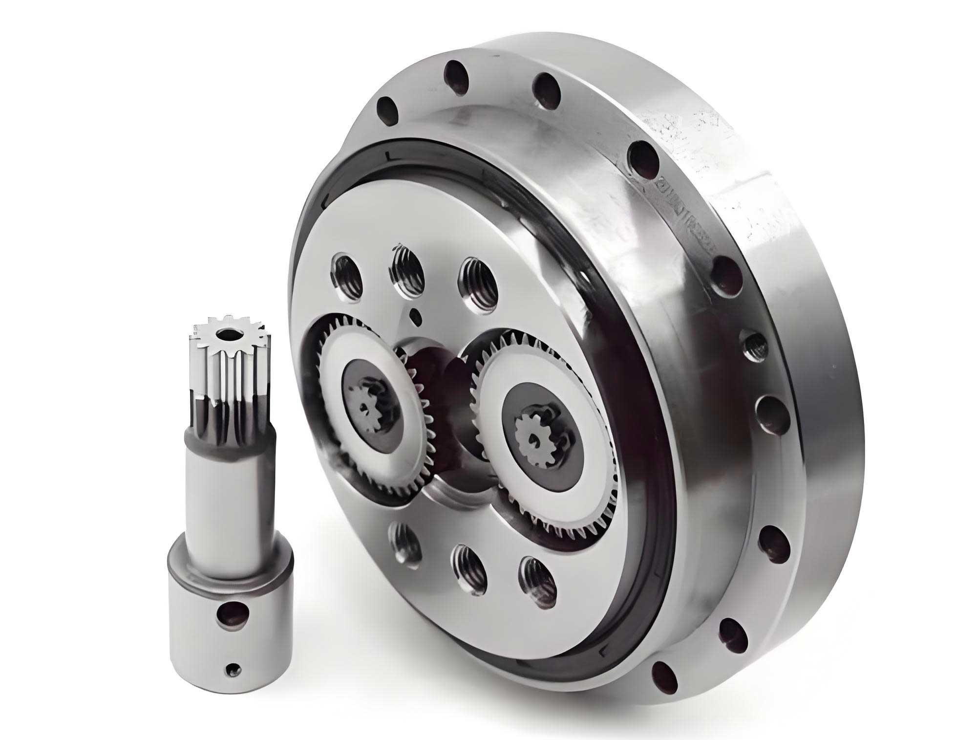
The dynamic performance and load distribution are critical. The force analysis on the cycloidal wheel and the pins is complex, involving Hertzian contact stresses. The maximum contact pressure $P_{max}$ between a cycloidal wheel lobe and a cylindrical pin can be estimated using the Hertz contact theory for parallel cylinders:
$$ P_{max} = \sqrt{\frac{F E^*}{\pi L R^*}} $$
where $F$ is the normal load per unit length, $L$ is the effective contact length, $E^*$ is the equivalent Young’s modulus, and $R^*$ is the equivalent radius of curvature. The equivalent modulus is given by:
$$ \frac{1}{E^*} = \frac{1 – \nu_1^2}{E_1} + \frac{1 – \nu_2^2}{E_2} $$
and the equivalent radius by:
$$ \frac{1}{R^*} = \frac{1}{R_1} \pm \frac{1}{R_2} $$
where $E_1, E_2$, $\nu_1, \nu_2$, and $R_1, R_2$ are the Young’s moduli, Poisson’s ratios, and radii of the two contacting bodies (cycloid lobe and pin), respectively. The sign depends on the convex/concave nature of the contact. Proper design ensures this pressure is well below the material’s fatigue limit for infinite life. This contact stress is a primary factor in the longevity and reliability of a rotary vector reducer.
The manufacturing precision required is astronomical. Key components like the cycloidal gear, the crankshaft, and the housing demand micron-level tolerances and super-finished surfaces. The following table summarizes critical tolerances for a high-performance rotary vector reducer:
| Component | Critical Feature | Typical Tolerance (µm) | Surface Finish Ra (µm) |
|---|---|---|---|
| Cycloidal Disk | Lobe profile | ± 3 | 0.2 – 0.4 |
| Needle Pins | Diameter consistency | ± 1 | 0.1 – 0.2 |
| Crankshaft | Eccentricity & Journal roundness | ± 2 | 0.1 |
| Main Housing | Bore concentricity | 5 (TIR) | 0.4 – 0.8 |
Material selection is equally vital. Components are typically forged from high-grade alloy steels like SCM415 or 20CrMnTi, followed by sophisticated heat treatment processes such as carburizing and quenching to achieve a hard, wear-resistant surface and a tough, fatigue-resistant core. The table below contrasts common materials and treatments:
| Component | Material | Core Hardness (HRC) | Surface Hardness (HRC) | Heat Treatment |
|---|---|---|---|---|
| Cycloidal Disk | 20CrMnTi | 28-32 | 58-62 | Carburizing (0.8-1.2mm depth) |
| Pin Gear (Housing) | GCr15 Bearing Steel | 58-62 (through-hardened) | 58-62 | Quenching & Tempering |
| Input Planetary Gears | SCM415 | 30-35 | 58-62 | Carburizing |
| Crankshaft | 42CrMo | 28-32 | 50-55 | Induction Hardening on journals |
The pursuit of performance mirrors concepts found in polymer science, such as the devulcanization of rubber. In that field, the efficiency of reclamation is measured by the reduction in crosslink density ($\nu$) and the increase in sol fraction ($S$). Similarly, the performance of a rotary vector reducer can be degraded by the “breaking” of its precision geometry through wear or fatigue. The wear rate, analogous to a scission rate in polymers, can be modeled. A fundamental parameter is the specific wear rate $k$, defined by the Archard wear equation:
$$ V = k \frac{F_N s}{H} $$
where $V$ is the wear volume, $F_N$ is the normal load, $s$ is the sliding distance, and $H$ is the hardness of the softer material. For a rotary vector reducer, minimizing $k$ through optimal material pairing and lubrication is the goal. Lubrication itself is a science, requiring grease with extreme pressure (EP) additives, high base oil viscosity, and excellent mechanical stability. The life calculation often follows a modified bearing life formula, such as:
$$ L_{10} = \left( \frac{C}{P} \right)^p \times 10^6 \text{ revolutions} $$
where $L_{10}$ is the rated life (90% survival), $C$ is the dynamic load rating, $P$ is the equivalent dynamic load, and $p$ is an exponent (typically 10/3 for roller contacts). The equivalent load $P$ for a rotary vector reducer must account for complex multi-directional forces and moments:
$$ P = f(F_{ra}, F_{ax}, M) $$
where $F_{ra}$ is radial force, $F_{ax}$ is axial force, and $M$ is the tilting moment. Manufacturers derive complex empirical formulas to calculate this.
Backlash, the lost motion between input and output under load reversal, is a critical performance metric for a rotary vector reducer in robotics. It is the sum of clearances in all mechanical interfaces. Minimizing it requires not just precision manufacturing but also preloading strategies. The total backlash $\beta_{total}$ can be expressed as a root-sum-square (RSS) of individual contributors under certain assumptions:
$$ \beta_{total} \approx \sqrt{\beta_{cycloid-pin}^2 + \beta_{bearing}^2 + \beta_{spline}^2} $$
where $\beta_{cycloid-pin}$ is the clearance in the cycloid-pin meshing, $\beta_{bearing}$ is the clearance in the support bearings, and $\beta_{spline}$ is the clearance in the output mechanism. High-precision units achieve backlash values below 1 arcmin.
Thermal management is another crucial aspect. During operation, power losses (primarily from friction) generate heat, raising the internal temperature. This can affect lubricant viscosity, clearances, and material properties. The steady-state temperature rise $\Delta T$ can be approximated by a simple thermal balance:
$$ P_{loss} = h A \Delta T $$
where $P_{loss}$ is the total power loss (in Watts), $h$ is the effective heat transfer coefficient, $A$ is the surface area for heat dissipation, and $\Delta T$ is the temperature rise above ambient. Power loss itself has components: load-dependent loss $P_L$ and no-load loss $P_0$ (from churning and seal friction). It can be modeled as:
$$ P_{loss} = P_0 + \left( \frac{T_{out}}{T_{rated}} \right)^\alpha P_{L,rated} $$
where $T_{out}$ is output torque, $T_{rated}$ is rated torque, and $\alpha$ is an exponent often near 1.5 to 2.
The design and analysis process heavily rely on advanced tools. Finite Element Analysis (FEA) is used for stress, deformation, and modal analysis. Multi-body dynamics (MBD) software simulates the complex motion and forces under dynamic loads. The following table outlines typical simulation scopes for a rotary vector reducer:
| Analysis Type | Purpose | Key Outputs |
|---|---|---|
| Static Structural FEA | Assess stress & deformation under peak load | Von Mises stress, Safety factor, Deflection maps |
| Modal Analysis | Determine natural frequencies & mode shapes | First 5-10 natural frequencies, Mode shapes |
| Transient Dynamic Analysis | Simulate shock loads or start/stop cycles | Time-history of stress, force, acceleration |
| Multi-body Dynamics (MBD) | Model full mechanism with contacts & joints | Load spectra on all parts, Kinematic accuracy, Dynamic forces |
| Thermal Analysis | Predict operating temperature distribution | Steady-state temperature field, Hot spots |
Testing and validation are where theory meets reality. A comprehensive test regimen for a rotary vector reducer includes life testing, efficiency mapping, torsional stiffness measurement, backlash measurement, and noise/vibration testing. Torsional stiffness $K_t$ is measured by applying a gradually increasing torque $T$ and measuring the angular deflection $\theta$:
$$ K_t = \frac{dT}{d\theta} \quad \text{[Nm/rad]} $$
This curve is often non-linear, with a lower initial stiffness due to taking up clearances, then becoming very linear and high. Efficiency $\eta$ is measured as the ratio of output power to input power across the torque and speed range:
$$ \eta(T, \omega) = \frac{T_{out} \cdot \omega_{out}}{T_{in} \cdot \omega_{in}} \times 100\% $$
where $\omega_{in}$ and $\omega_{out}$ are input and output angular speeds, respectively. A full efficiency map is a 3D plot or contour map that is essential for system integration.
The market evolution and future trends for the rotary vector reducer point towards even higher performance, integration, and intelligence. Direct-drive technologies pose a challenge, but for applications requiring immense torque density and rigidity, the rotary vector reducer remains unrivaled. Future developments include the use of advanced materials like ceramic composites for wear parts, integrated sensors for condition monitoring, and digital twins for predictive maintenance. The core mathematics of the cycloidal drive may remain constant, but its realization continues to evolve. The mathematical optimization of the cycloid profile itself is an area of ongoing research, often involving modifications to the standard profile to optimize contact stress and manufacturing. A modified profile might be defined by a parametric equation that introduces correction coefficients $\epsilon_1$ and $\epsilon_2$:
$$ x(\phi) = (R_p + \epsilon_1) \cos(\phi) – r_r \cos(\phi + \psi) – a \cos(Z_c \phi) $$
$$ y(\phi) = (R_p + \epsilon_2) \sin(\phi) – r_r \sin(\phi + \psi) – a \sin(Z_c \phi) $$
where $R_p$ is the pin circle radius, $r_r$ is the pin radius, $a$ is the eccentricity, $Z_c$ is the number of lobes, $\phi$ is the input angle, and $\psi$ is a phase angle. The coefficients $\epsilon_1$ and $\epsilon_2$ are optimized to equalize load distribution across pins.
In conclusion, the mastery of the rotary vector reducer is a symphony of disciplines: precision mechanics, material science, tribology, thermal dynamics, and advanced manufacturing. Its development, much like the reclamation and optimization of complex polymer networks, requires a deep understanding of the relationship between microstructure (or geometry), processing, and final performance. Each advancement in tolerance control, heat treatment, lubricant formulation, or profile design pushes the boundaries of what is possible in robotic articulation and precision motion control. The journey of perfecting this key component is a continuous one, driven by the relentless pursuit of higher efficiency, greater reliability, and more compact power density in the ever-evolving world of automation.