
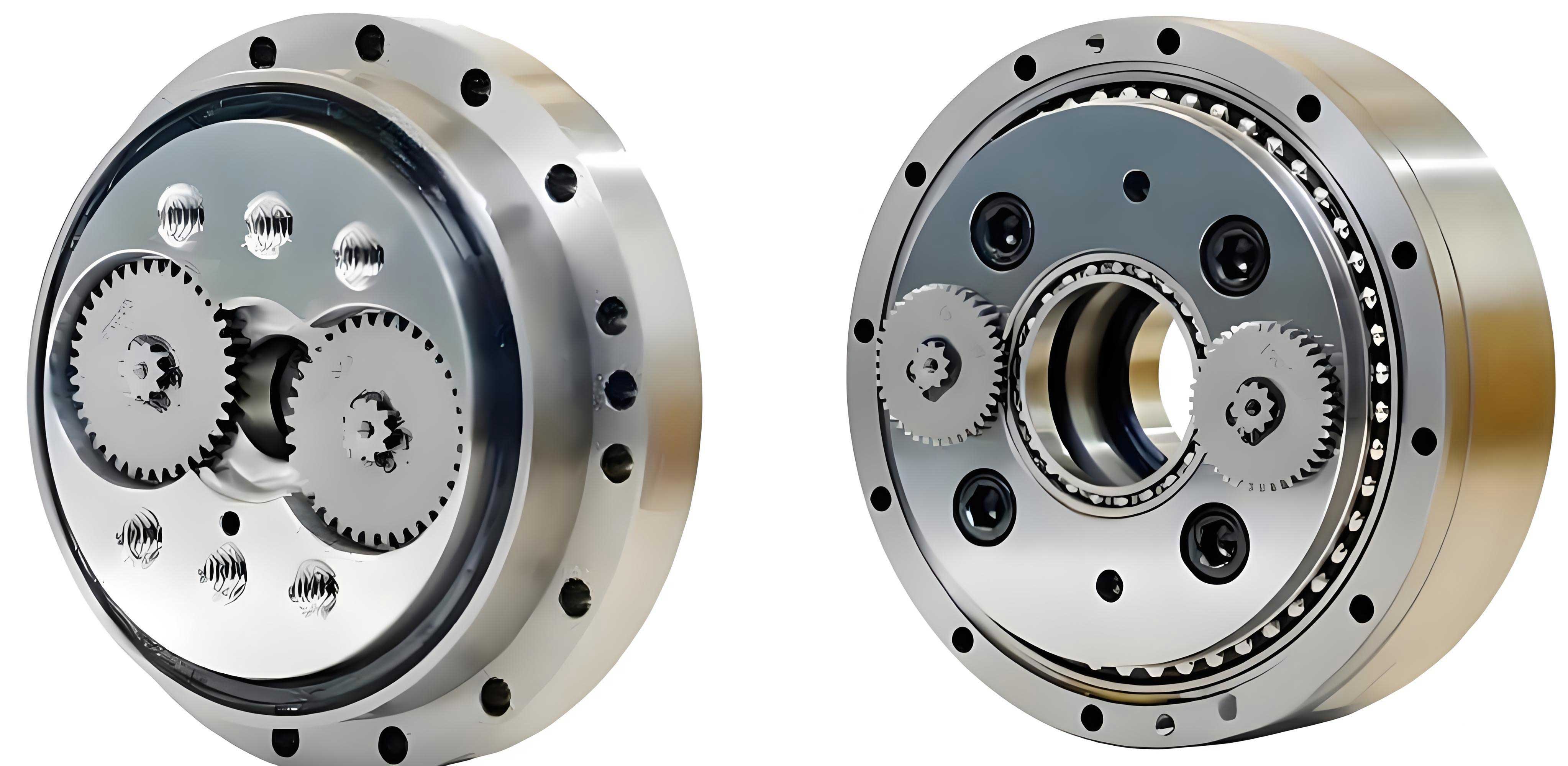
The relentless pursuit of precision, compactness, and reliability in modern robotics, medical devices, and aerospace systems has cemented the Rotary Vector (RV) reducer as a critical power transmission component. Its unique dual-stage architecture, combining a planetary gear stage with a cycloidal speed reducer, offers exceptional advantages: high reduction ratios, substantial torque capacity, remarkable torsional stiffness, and minimal backlash. Achieving these performance benchmarks, particularly a transmission error often specified to be within one arc-minute, imposes extraordinarily stringent requirements on the manufacturing and, crucially, the final assembly process. Each RV reducer is a symphony of precision parts—cycloidal disks, crankshafts, needle bearings, and the main housing (center frame)—where the cumulative effect of micro-scale geometric deviations directly impacts the final output quality.
The traditional paradigm of achieving such precision through complete interchangeability—machining every component to a near-perfect tolerance—is economically prohibitive for mass production. It forces machining processes to operate at the very limits of capability, drastically increasing cost and scrap rates. The classical alternative, group matching (or selective assembly), offers a more economical path. Components are machined to wider, more cost-effective tolerances, measured, sorted into bins based on their actual dimensions, and then assembled from corresponding bins. While useful, this method suffers from significant inherent flaws. Its efficacy is entirely dependent on the statistical distribution of the manufactured parts. If the distributions of mating components (e.g., the center distance of holes in the housing and the center distance of holes in the cycloidal disk set) are not perfectly aligned, substantial quantities of parts become “orphans,” leading to high rates of non-assembled inventory. Furthermore, for medium or small batch sizes, finding the absolute maximum number of valid assemblies from a given pool of parts is computationally blind and often suboptimal with a simple grouping strategy.
This is where the power of computational optimization and discrete mathematics comes to the fore. By reframing the assembly matching problem as a combinatorial graph theory problem, we can systematically search for the global optimum—the maximum number of valid assemblies from a given set of components. Among various optimization models, the theory of bipartite graph matching provides an elegant, powerful, and computationally efficient framework perfectly suited for pairing two distinct sets of items, which is the core of many RV reducer sub-assembly tasks.
Bipartite Graph Matching: A Formal Foundation for Optimal Pairing
At its heart, the challenge of selecting which center frame to pair with which cycloidal disk set is a “marriage problem.” We have two distinct groups, and we wish to create as many compatible pairs as possible. Bipartite graph theory formalizes this. A bipartite graph, denoted as $G = (X, Y, E)$, is defined by two disjoint sets of vertices, $X$ and $Y$, and a set of edges $E$ where each edge connects a vertex in $X$ to a vertex in $Y$. No edge connects vertices within the same set. In our RV reducer assembly context:
- $X = \{x_1, x_2, …, x_m\}$ represents the set of available center frames.
- $Y = \{y_1, y_2, …, y_n\}$ represents the set of available cycloidal disk sets.
- An edge $e = (x_i, y_j)$ exists in $E$ if and only if the dimensional difference between center frame $i$ and disk set $j$ is within the specified allowable assembly tolerance (e.g., $\pm 3 \mu m$). This is the fundamental compatibility criterion.
The core concept is that of a matching. A matching $M$ is a subset of edges $M \subseteq E$ such that no two edges in $M$ share a common vertex. In practical terms, a matching represents a valid assembly plan where each part is used at most once. The size of a matching, $|M|$, is the number of assembled pairs. Our objective is to find a maximum matching $M_{max}$—a matching of the largest possible size for the graph $G$. This directly corresponds to maximizing the yield from our inventory of RV reducer components.
To solidify these definitions, consider the following table which summarizes key graph-theoretic concepts and their assembly analogs:
| Graph Theory Term | Mathematical Symbol | Assembly Interpretation |
|---|---|---|
| Bipartite Graph | $G=(X, Y, E)$ | The entire pool of parts and all possible compatible pairs. |
| Vertex (in X or Y) | $x_i$, $y_j$ | An individual physical component (e.g., a specific center frame). |
| Edge | $e = (x_i, y_j)$ | A potential valid assembly between two specific components. |
| Matching | $M \subseteq E$ | A set of confirmed, non-conflicting assemblies (a build plan). |
| Maximum Matching | $M_{max}$ | The build plan that results in the highest number of finished RV reducers. |
| Free/Unmatched Vertex | $v \notin V(M)$ | A leftover component not used in the current matching/plan. |
A pivotal theorem in matching theory, Berge’s Lemma, provides the mechanism to find a maximum matching. It states that a matching $M$ is not maximum if and only if there exists an augmenting path relative to $M$. An augmenting path is a sequence of edges that starts and ends at free (unmatched) vertices, and alternately travels through edges not in $M$ and edges in $M$. The power of this path is that by “flipping” the status of the edges along it (i.e., removing the matched edges on the path from $M$ and adding the unmatched ones), we increase the size of the matching by exactly one. This operation is the symmetric difference: $M’ = M \oplus P = (M \cup P) – (M \cap P)$.
Therefore, the algorithm to find the maximum matching starts with an empty or arbitrary matching and iteratively searches for and augments along these paths until none exist, guaranteeing optimality.
The Hungarian Algorithm: A Systematic Path to Maximum Yield
The Hungarian Algorithm, developed by Kuhn and based on the work of König and Egerváry, is a classic and efficient procedure for finding a maximum matching in a bipartite graph. It operationalizes the search for augmenting paths. The algorithm can be effectively implemented using an adjacency matrix representation of the compatibility graph, making it highly suitable for computer automation.
Let the number of center frames be $m$ and cycloidal disk sets be $n$. We construct an $m \times n$ binary matrix $A$, where:
$$A_{ij} = \begin{cases}
1 & \text{if } |L_{1_i} – L_{2_j}| \le \delta \\
0 & \text{otherwise}
\end{cases}$$
Here, $L_{1_i}$ is the center distance of the $i$-th frame, $L_{2_j}$ is the center distance of the $j$-th disk set, and $\delta$ is the assembly tolerance (e.g., 0.003 mm). This matrix $A$ fully encapsulates the bipartite graph $G$.
The steps of the Hungarian algorithm (adapted for maximum cardinality matching) are as follows:
- Initialization: Begin with an empty matching $M = \varnothing$.
- Iteration: For each unmatched vertex $u$ in set $X$:
- Perform a modified graph search (Depth-First or Breadth-First) from $u$ to find an augmenting path $P$ to an unmatched vertex in $Y$. This search must respect the alternating path condition (edge not in $M$, then edge in $M$, etc.).
- If an augmenting path $P$ is found, update the matching: $M \leftarrow M \oplus P$.
- If no path is found, $u$ remains unmatched.
- Termination: The algorithm terminates when all vertices in $X$ have been processed. The resulting matching $M$ is a maximum matching.
The computational complexity of a straightforward implementation is $O(|E| \cdot |V|)$, where $|V| = m+n$. For sparse graphs (where each part is compatible with only a subset of others), more advanced algorithms like the Hopcroft-Karp algorithm offer a better worst-case complexity of $O(\sqrt{|V|} \cdot |E|)$, making them scalable for very large inventories of RV reducer components.
Application to RV Reducer Assembly: A Concrete Case Study
Consider the sub-assembly of an RV-20E type reducer, focusing on the critical “parallelogram mechanism” formed by the center frame and the cycloidal disk pair. The functional requirement is that the center distance of the bearing bores in the frame ($L_1$) must be as close as possible to the center distance of the bearing bores in the disk set ($L_2$) to prevent pre-loading or binding of the intermediate needle bearings. The design nominal value is 55.000 mm, with a manufacturing tolerance of ±0.023 mm. The allowable assembly mismatch $\delta$ is set to 0.003 mm.
Suppose we have the following measured data from the production batch:
| Center Frame ID | $L_1$ (mm) | Cycloidal Disk Set ID | $L_2$ (mm) |
|---|---|---|---|
| CF-01 | 55.007 | CD-01 | 55.003 |
| CF-02 | 55.007 | CD-02 | 54.999 |
| CF-03 | 54.988 | CD-03 | 54.994 |
| CF-04 | 55.000 | CD-04 | 55.005 |
| CF-05 | 54.979 | CD-05 | 55.001 |
| CF-06 | 54.992 | CD-06 | 54.998 |
| CF-07 | 54.995 | CD-07 | 54.995 |
| CF-08 | 54.999 | CD-08 | 54.980 |
| CF-09 | 54.995 | CD-09 | 55.010 |
| CF-10 | 54.999 | CD-10 | 54.999 |
The first step is to build the compatibility matrix $A$ based on the rule $|L_1 – L_2| \le 0.003$. Applying the Hungarian algorithm to this matrix yields the optimal matching. The result is a maximum matching of size 9, meaning 9 complete assemblies can be formed from these 10 components of each type. A traditional group matching approach, dividing parts into bins of width 0.006 mm (e.g., 54.997-55.003, etc.), would likely result in fewer valid pairs due to distribution mismatches and the rigid binning structure.
| Matched Pair # | Center Frame | Cycloidal Disk Set | Dimensional Difference (mm) |
|---|---|---|---|
| 1 | CF-01 | CD-04 | 0.002 |
| 2 | CF-02 | CD-09 | -0.003 |
| 3 | CF-04 | CD-01 | -0.003 |
| 4 | CF-05 | CD-08 | -0.001 |
| 5 | CF-06 | CD-03 | -0.002 |
| 6 | CF-07 | CD-06 | -0.003 |
| 7 | CF-08 | CD-02 | 0.000 |
| 8 | CF-09 | CD-07 | 0.000 |
| 9 | CF-10 | CD-05 | -0.002 |
This demonstrates the core advantage: the algorithm actively seeks the best global pairing combination, potentially utilizing parts that would be stranded in different groups under a simple sorting scheme, thereby maximizing the output of functional RV reducers and minimizing waste.
Comparative Analysis and Performance Validation
To quantitatively evaluate the superiority of the bipartite graph matching approach over traditional group matching, a Monte Carlo simulation is instructive. We model the manufacturing process by assuming the critical dimensions of two mating component types, Part A (e.g., center frame) and Part B (e.g., disk set), follow normal distributions: $L_A \sim N(\mu_A, \sigma_A^2)$ and $L_B \sim N(\mu_B, \sigma_B^2)$. The matching tolerance is $\delta$. We define the key performance metric, Matching Rate $f(p)$, as:
$$f(p) = \frac{n_p}{N} \times 100\%$$
where $n_p$ is the number of successfully matched pairs (the size of the maximum matching) and $N$ is the total number of components available for assembly (typically $N = |X| + |Y|$, or the smaller of the two sets for rate calculation).
We simulate batches with varying population sizes (from 10 to 200 parts per type) and under different distribution scenarios (varying means $\mu$ and standard deviations $\sigma$). For each scenario, we compare the matching rate achieved by the optimal bipartite matching algorithm against a standard group matching strategy with a fixed bin width of $2\delta$.
The simulation parameters are summarized below:
| Parameter | Value / Range |
|---|---|
| Components per batch (|X|, |Y|) | 10 to 200 |
| Assembly Tolerance ($\delta$) | 0.003 mm |
| Nominal Dimension ($\mu_A, \mu_B$) | 30.000 mm |
| Standard Deviation ($\sigma_A, \sigma_B$) | 0.005 mm to 0.030 mm |
| Group Matching Bin Width | 0.006 mm ($2\delta$) |
The results consistently demonstrate the advantage of the graph-based method:
- Consistent Superiority: Across all tested conditions—balanced distributions ($\mu_A = \mu_B$), shifted means ($\mu_A \neq \mu_B$), and varying process capabilities (different $\sigma$)—the bipartite matching algorithm achieves a higher matching rate than the group method.
- Performance Gap: The magnitude of improvement ranges from approximately 6% to as high as 25% in matching rate. The largest gains are observed when the part distributions are not perfectly aligned or when the process variation ($\sigma$) is large relative to the assembly tolerance ($\delta$). This is precisely the real-world scenario where traditional group matching struggles with orphaned parts.
- Robustness to Distribution: The bipartite matching algorithm does not assume any specific distribution of parts. It works directly on the measured data, making it robust to non-normal or skewed distributions common in machining processes.
- Inventory Efficiency: For a manufacturer, this increase in matching rate translates directly to higher throughput, lower work-in-process inventory, and reduced scrap. More RV reducers are assembled from the same input materials.
Beyond Simple Pairs: Extensions and Industrial Application
The bipartite matching model, while powerful for pairwise assembly, represents the foundational building block for more complex RV reducer assembly challenges. A complete RV reducer involves multiple interrelated matching problems: crankshaft pins to needle bearings, needle bearings to cycloidal disk holes, and the final fit of the planetary stage. This can be modeled as a multi-stage or multi-layer matching problem.
One advanced approach is to construct a multi-partite graph or use sequential optimization. For instance, after solving the center-frame-to-disk-set matching, the resulting sub-assemblies (now treated as new vertices) can be matched with appropriate crankshafts in a subsequent bipartite graph, potentially with different compatibility constraints. While finding a global optimum for a multi-layer problem is more complex (and can be NP-hard in general formulations), the bipartite matching solution at each stage often provides a very high-quality, feasible assembly plan that is superior to any manual or grouped approach.
Integration into a modern smart factory is straightforward. The process flow would be:
- Digital Measurement: All critical components of the RV reducer are measured automatically, and their as-built dimensions are stored in a database.
- Graph Construction: For a planned assembly batch, the system retrieves the dimensions and constructs the relevant compatibility matrices based on engineering tolerances.
- Optimal Matching Execution: The Hungarian or Hopcroft-Karp algorithm is executed to find the maximum matching(s).
- Instruction Dispatch: The optimal pairing list is sent to the assembly station, guiding the operator or robot to pick and assemble the specified components (e.g., “Assemble Center Frame CF-07 with Disk Set CD-06”).
- Feedback Loop: Data on matching rates and leftover parts feeds back to the machining department for continuous process improvement.
The implications extend beyond the RV reducer itself. This methodology is universally applicable to any precision assembly where selective fitting is required: fuel injector nozzles, hydraulic valve spools and sleeves, high-precision bearing assemblies, and optical lens elements. The core principle of using combinatorial optimization to maximize yield from components produced at economic tolerances is a key enabler for high-quality, cost-effective advanced manufacturing.
In conclusion, the transition from heuristic, distribution-dependent group matching to algorithm-driven bipartite graph maximum matching represents a significant leap forward in precision assembly strategy. For RV reducer manufacturers and other precision engineering fields, adopting this approach directly addresses the economic paradox of precision—it allows the use of cost-effective manufacturing processes while ensuring the final product meets the most stringent performance requirements through intelligent, optimal combinatorial assembly. This synergy of classical graph theory with modern computational power provides a robust, scalable, and superior framework for maximizing quality and efficiency in the production of complex mechanical systems like the RV reducer.