
Enhancing the operational precision of CNC machine tools is a persistent challenge in advanced manufacturing. The rotary table, a critical functional component in multi-axis machining centers, directly influences the overall machining accuracy and stability of the machine tool. Among various drive configurations, the worm gear and worm mechanism remains widely adopted in precision turntables due to its high reduction ratio, compact design, and self-locking capability. However, the final positioning accuracy of the turntable is not solely a function of the worm gears manufacturing quality but is critically determined by the accumulation and propagation of geometric errors throughout the entire transmission chain. Factors such as assembly misalignments, bearing runout, and structural deformations under load all contribute to the output error at the worktable. This necessitates a holistic, system-level approach to error modeling and precision design. Traditional piecemeal analysis often falls short of capturing the complex interplay of multiple error sources. Therefore, this study focuses on establishing a comprehensive theoretical framework, based on Multi-Body System (MBS) theory, for the error modeling, sensitivity analysis, and precision allocation of worm gear-driven precision turntables, providing a solid foundation for their optimal design and industrial application.
Introduction and Background
The pursuit of higher machining accuracy drives continuous innovation in the design and control of key machine tool components. Precision rotary tables are indispensable for complex multi-sided machining operations. Their performance, particularly the angular positioning accuracy and repeatability, is paramount. The worm gear and worm drive offers a reliable solution for transmitting motion and torque from the servo motor to the large-diameter worktable. Despite its advantages, the kinematic chain involving the motor, coupling, worm gears pair, anti-backlash mechanism, and the final worktable is susceptible to numerous geometric errors. These errors, stemming from manufacturing tolerances and assembly processes, propagate through the system, culminating in a deviation of the tool center point or workpiece location from its ideal position.
Previous research has explored various aspects of turntable and machine tool accuracy. Studies have applied Multi-Body System theory to model errors in dual-worm drives, three-axis simulators, and five-axis machines, often focusing on topological description and error element identification. Others have investigated sensitivity analysis methods or proposed error measurement techniques using laser interferometers and polygon mirrors. A common gap in much of this work is the lack of a complete, quantitative, and structured methodology that links the fundamental error sources within a worm gears transmission system directly to the final output error through a mathematically rigorous model, followed by a systematic procedure for identifying dominant error sources and allocating tolerances. This paper aims to address this gap. By leveraging the formalisms of MBS theory, we construct a complete mathematical model for error propagation in a worm gear turntable, perform a detailed sensitivity analysis using differential methods to identify key error contributors, and demonstrate the application of this framework in a practical precision design case, ultimately verifying the results through experimental testing.
Fundamentals of Multi-Body System Theory for Error Modeling
Multi-Body System theory provides a generalized and systematic methodology for modeling the kinematics and dynamics of complex mechanical systems. Any mechanical system can be abstracted into a set of rigid or flexible bodies connected by joints that define their relative degrees of freedom. For precision error analysis, the kinematic aspect is primary. The core mathematical tool is the homogeneous transformation matrix, which describes the position and orientation (pose) of one coordinate frame relative to another.
Consider two adjacent bodies, body i and body j, in a kinematic chain. Let \( ^iP \) represent the coordinates of a point P expressed in the coordinate frame attached to body i. Its coordinates in the frame of body j, denoted \( ^jP \), are obtained through a sequence of transformations:
$$ ^jP = \mathbf{T}_{i}^{j} \cdot ^iP $$
Where \( \mathbf{T}_{i}^{j} \) is the 4×4 homogeneous transformation matrix from frame i to frame j. In the context of error modeling for a precision mechanism, this ideal transformation is decomposed into components representing nominal design, geometric errors, ideal motion, and motion errors. The general form for the actual transformation between two adjacent bodies is:
$$ \mathbf{T}_{actual} = \mathbf{T}_{P} \cdot \mathbf{T}_{PE} \cdot \mathbf{T}_{S} \cdot \mathbf{T}_{SE} $$
Where:
\( \mathbf{T}_{P} \): Nominal relative position (constant, defined by design).
\( \mathbf{T}_{PE} \): Position error matrix (constant geometric errors like squareness, offset).
\( \mathbf{T}_{S} \): Ideal relative motion matrix (function of joint variable, e.g., rotation angle).
\( \mathbf{T}_{SE} \): Motion error matrix (errors dependent on motion, like axis tilt and radial runout).
This decomposition allows for the explicit inclusion of all potential error sources at each interface in the kinematic chain. The topology of the system is described using a low-order body array, which defines the sequence of bodies from the fixed base (body 0) to the terminal body (e.g., the workpiece or tool).
Worm Gear Turntable Transmission Chain and Topological Structure
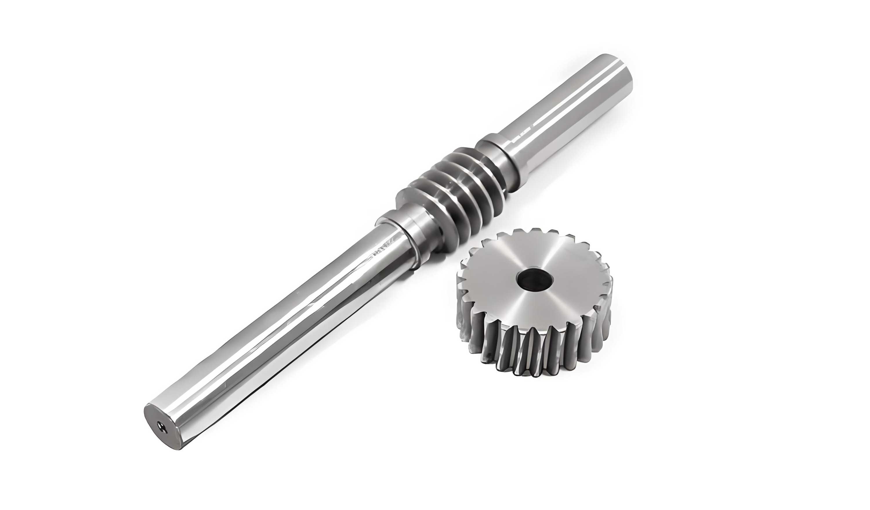
The object of study is a horizontal machining center’s worm gear-driven precision rotary table. Its main transmission sequence, constituting the primary accuracy chain, is as follows: Servo Motor (mounted on a slide) → Coupling → Worm Shaft System → Worm Wheel System (integrated with an anti-backlash mechanism) → Worktable System (via a face gear or direct coupling) → Load (Workpiece).
To apply MBS theory, this physical chain is abstracted into a multi-body system with five main bodies: \( K_0 \) (Slide/Base), \( K_1 \) (Worm Shaft System), \( K_2 \) (Worm Wheel System), \( K_3 \) (Worktable System), and \( K_4 \) (Load). Each body \( K_n \) has a coordinate frame \( O_n-X_nY_nZ_n \) attached to it. The kinematic relationship is an open-loop chain: \( K_0 \rightarrow K_1 \rightarrow K_2 \rightarrow K_3 \rightarrow K_4 \). The ideal motion is defined by rotation angles: \( \alpha \) for the worm shaft (body \( K_1 \)) relative to the slide, \( \beta \) for the worm wheel (body \( K_2 \)), and \( \gamma \) for the worktable (body \( K_3 \)). The load is assumed to be fixed relative to the worktable. The core modeling task is to derive the actual position of a point on the load (e.g., its axis vector) relative to the inertial base frame \( K_0 \), accounting for all errors along the chain.
Comprehensive Geometric Error Modeling
The error model is built by defining the characteristic matrices for each adjacent body pair according to the structure and error sources of the worm gears turntable. The primary geometric error sources considered are classified into two categories: position errors (constant misalignments like perpendicularity) and motion errors (angular and translational deviations during rotation).
Definition of Key Error Elements:
For a rotation axis, several error components exist. Let the nominal axis of rotation between body j and body i be along direction n. The associated errors are:
– Perpendicularity Errors (\( \varepsilon \)): Constant angular misalignment of the axis of rotation relative to a reference axis of the previous body.
– Tilt Error Motions (\( \delta_x, \delta_y \)): Angular error motions of the rotating body, projected onto axes perpendicular to the nominal rotation axis.
– Axial Error Motion (\( \delta_z \)): Translational error motion along the nominal rotation axis.
– Load Mounting Errors (\( \sigma \)): Angular misalignments when installing the load onto the worktable.
The specific error elements for the worm gear turntable are listed in the table below.
| Body Pair | Error Type | Symbol | Description |
|---|---|---|---|
| \(K_0\)-\(K_1\) (Worm Shaft) | Perpendicularity | \( \varepsilon_{x0}^{(y1)}, \varepsilon_{z0}^{(y1)} \) | Worm shaft axis (Y1) sq. to X0 and Z0 of slide. |
| Motion Error | \( \delta_{x}^{(y1)}, \delta_{y}^{(y1)} \) | Tilt error of worm shaft. | |
| \( \delta_{z}^{(y1)} \) | Axial error of worm shaft. | ||
| \(K_1\)-\(K_2\) (Worm Wheel) | Perpendicularity | \( \varepsilon_{x1}^{(z2)}, \varepsilon_{y1}^{(z2)} \) | Worm wheel axis (Z2) sq. to X1 and Y1 of worm shaft body. |
| Motion Error | \( \delta_{x}^{(z2)}, \delta_{y}^{(z2)} \) | Tilt error of worm wheel. | |
| \( \delta_{z}^{(z2)} \) | Axial error of worm wheel. | ||
| \(K_2\)-\(K_3\) (Worktable) | Perpendicularity | \( \varepsilon_{x2}^{(z3)}, \varepsilon_{y2}^{(z3)} \) | Worktable axis (Z3) sq. to X2 and Y2 of worm wheel body. |
| Motion Error | \( \delta_{x}^{(z3)}, \delta_{y}^{(z3)} \) | Tilt error of worktable. | |
| \( \delta_{z}^{(z3)} \) | Axial error of worktable. | ||
| \(K_3\)-\(K_4\) (Load) | Mounting Error | \( \sigma_{x}^{(x4)}, \sigma_{y}^{(y4)}, \sigma_{z}^{(z4)} \) | Angular misalignment of load relative to worktable. |
Derivation of Characteristic Matrices:
Using the small-angle approximation, the characteristic matrices for each adjacent body pair are constructed. The rotation matrix \( rot(\mathbf{n}, \theta) \) represents a rotation of angle \( \theta \) about axis vector \( \mathbf{n} \).
For the pair \( K_0\)-\(K_1 \) (Worm shaft rotation about \( Y_0 \)):
Nominal position: \( \mathbf{T}_{01P} = \mathbf{I}_{4\times4} \)
Position error: \( \mathbf{T}_{01PE} = rot(x_0, \varepsilon_{x0}^{(y1)}) \cdot rot(z_0, \varepsilon_{z0}^{(y1)}) \)
Ideal motion: \( \mathbf{T}_{01S} = rot(y_0, \alpha) \)
Motion error: \( \mathbf{T}_{01SE} = rot(x_0, \delta_{x}^{(y1)}) \cdot rot(y_0, \delta_{y}^{(y1)}) \cdot rot(z_0, \delta_{z}^{(y1)}) \)
Similarly, for \( K_1\)-\(K_2 \) (Worm wheel rotation about \( Z_1 \)):
\( \mathbf{T}_{12P} = \mathbf{I} \)
\( \mathbf{T}_{12PE} = rot(x_1, \varepsilon_{x1}^{(z2)}) \cdot rot(y_1, \varepsilon_{y1}^{(z2)}) \)
\( \mathbf{T}_{12S} = rot(z_1, \beta) \)
\( \mathbf{T}_{12SE} = rot(x_1, \delta_{x}^{(z2)}) \cdot rot(y_1, \delta_{y}^{(z2)}) \cdot rot(z_1, \delta_{z}^{(z2)}) \)
For \( K_2\)-\(K_3 \) (Worktable rotation about \( Z_2 \)):
\( \mathbf{T}_{23P} = \mathbf{I} \)
\( \mathbf{T}_{23PE} = rot(x_2, \varepsilon_{x2}^{(z3)}) \cdot rot(y_2, \varepsilon_{y2}^{(z3)}) \)
\( \mathbf{T}_{23S} = rot(z_2, \gamma) \)
\( \mathbf{T}_{23SE} = rot(x_2, \delta_{x}^{(z3)}) \cdot rot(y_2, \delta_{y}^{(z3)}) \cdot rot(z_2, \delta_{z}^{(z3)}) \)
For \( K_3\)-\(K_4 \) (Static load mounting):
\( \mathbf{T}_{34P} = \mathbf{I} \), \( \mathbf{T}_{34S} = \mathbf{I} \), \( \mathbf{T}_{34SE} = \mathbf{I} \)
\( \mathbf{T}_{34PE} = rot(x_3, \sigma_{x}^{(x4)}) \cdot rot(y_3, \sigma_{y}^{(y4)}) \cdot rot(z_3, \sigma_{z}^{(z4)}) \)
Total Error Model Formulation:
The ideal overall transformation from the load (body \( K_4 \)) to the base (body \( K_0 \)) is the product of the ideal motion and position matrices:
$$ \mathbf{T}_{ide} = \prod_{i=0}^{3} \left( \mathbf{T}_{i(i+1)P} \cdot \mathbf{T}_{i(i+1)S} \right) $$
The actual transformation includes all error matrices:
$$ \mathbf{T}_{act} = \prod_{i=0}^{3} \left( \mathbf{T}_{i(i+1)P} \cdot \mathbf{T}_{i(i+1)PE} \cdot \mathbf{T}_{i(i+1)S} \cdot \mathbf{T}_{i(i+1)SE} \right) $$
To quantify the output error, we consider a vector representing the orientation of the load axis. In the load’s own frame \( O_4 \), let this unit vector be \( \mathbf{e} = [0, 0, 1]^T \). Its representation in the base frame \( O_0 \) under ideal and actual conditions is:
$$ \mathbf{P}_{ide} = \mathbf{T}_{ide} \cdot \mathbf{e} $$
$$ \mathbf{P}_{act} = \mathbf{T}_{act} \cdot \mathbf{e} $$
The volumetric error vector \( \boldsymbol{\mu} \) at the load, expressed in the base coordinate system, is defined as the difference:
$$ \boldsymbol{\mu} = \begin{bmatrix} \mu_x \\ \mu_y \\ \mu_z \end{bmatrix} = \mathbf{P}_{act} – \mathbf{P}_{ide} $$
Substituting the derived matrices for \( \mathbf{T}_{act} \) and \( \mathbf{T}_{ide} \) into this equation yields the complete analytical error model for the worm gears precision turntable, explicitly relating the three-dimensional output error \( (\mu_x, \mu_y, \mu_z) \) to the 18 input error parameters \( (\varepsilon…, \delta…, \sigma…) \) and the motion commands \( (\alpha, \beta, \gamma) \).
Sensitivity Analysis and Identification of Key Error Sources
With the complex error model established, it is crucial to determine which error sources have the greatest impact on the final output precision. This guides cost-effective precision allocation during design and manufacturing. The method of function differentials (total derivative) is employed for sensitivity analysis.
Let the output error component \( \mu_k \) (where \( k = x, y, z \)) be a function of all \( m \) error source variables \( \theta_i \):
$$ \mu_k = f_k(\theta_1, \theta_2, …, \theta_m) $$
For small variations \( \Delta\theta_i \), the resulting change in \( \mu_k \) can be approximated by the first-order total differential:
$$ \Delta \mu_k \approx \sum_{i=1}^{m} \frac{\partial f_k}{\partial \theta_i} \Delta\theta_i $$
The partial derivative \( S_{ki} = \frac{\partial f_k}{\partial \theta_i} \) is defined as the sensitivity coefficient of output error \( \mu_k \) with respect to error source \( \theta_i \). It quantifies how much \( \mu_k \) changes per unit change in \( \theta_i \), assuming other errors are zero.
By taking the partial derivatives of the analytical error model \( \boldsymbol{\mu} = \mathbf{P}_{act} – \mathbf{P}_{ide} \) with respect to each error parameter, the complete sensitivity matrix can be derived. A normalized sensitivity index \( \lambda_{ki} \) is then calculated to compare the relative influence of different error sources across potentially different units and scales:
$$ \lambda_{ki} = \frac{|S_{ki}|}{\sum_{j=1}^{m} |S_{kj}|} $$
This index represents the fractional contribution of error source \( \theta_i \) to the sensitivity magnitude of output \( \mu_k \).
Applying this analysis to the worm gears turntable model and evaluating over a full range of motion (\( \alpha, \beta, \gamma \) from 0 to 360°), the average normalized sensitivity indices for each error component are computed. The results, highlighting the most influential error sources, are summarized below.
| Output Error Component | High-Impact Error Sources (Normalized Coefficient > 0.1) | Approx. Combined Influence |
|---|---|---|
| \( \mu_x \) (X-direction error) | \( \delta_{x}^{(z3)} \) (Worktable X-tilt), \( \sigma_{x}^{(x4)} \) (Load X-mounting error) | ~85% |
| \( \mu_y \) (Y-direction error) | \( \varepsilon_{z0}^{(y1)} \) (Worm shaft Z-perp.), \( \varepsilon_{y1}^{(z2)} \) (Worm wheel Y-perp.), \( \varepsilon_{x2}^{(z3)} \) (Worktable X-perp.), \( \delta_{z}^{(y1)} \) (Worm shaft axial), \( \delta_{y}^{(z2)} \) (Worm wheel Y-tilt), \( \delta_{y}^{(z3)} \) (Worktable Y-tilt), \( \sigma_{y}^{(y4)} \) (Load Y-mounting error) |
~95% |
| \( \mu_z \) (Z-direction error) | \( \varepsilon_{x0}^{(y1)} \) (Worm shaft X-perp.), \( \varepsilon_{x1}^{(z2)} \) (Worm wheel X-perp.), \( \delta_{x}^{(z3)} \) (Worktable X-tilt), \( \sigma_{x}^{(x4)} \) (Load X-mounting error) |
~92% |
The analysis reveals a critical insight: while all errors contribute, a subset is responsible for the majority of the output inaccuracy. For instance, the tilt error motions of the worktable (\( \delta_{x}^{(z3)}, \delta_{y}^{(z3)} \)) and the perpendicularity errors in the worm gears drive chain (\( \varepsilon_{z0}^{(y1)}, \varepsilon_{y1}^{(z2)} \)) are consistently dominant. This directs the designer’s focus: tightening tolerances or implementing error compensation for these specific parameters will yield the highest return on investment in terms of overall accuracy improvement.
Precision Allocation and Design Application
The sensitivity analysis provides the theoretical basis for a rational precision design process. The goal is to determine the allowable tolerance for each error source such that the final aggregate output error meets a specified target, often while considering manufacturing cost. The process can be outlined as follows:
- Set System-Level Accuracy Target: Define the maximum allowable volumetric error or, more commonly, angular positioning/repeatability error for the turntable (e.g., 4 arc-seconds).
- Error Budgeting: Using the error model and sensitivity indices, allocate portions of the total error budget to individual error sources. A common approach is to use the root-sum-square (RSS) method, assuming errors are statistically independent: $$ E_{total}^2 \approx \sum_{i=1}^{m} (S_i \cdot T_i)^2 $$ where \( E_{total} \) is the target output error, \( S_i \) is the effective sensitivity, and \( T_i \) is the tolerance to be assigned to error source \( i \). Higher sensitivity errors receive tighter tolerances.
- Map to Component Specifications: Translate the allocated error tolerances (angles in radians, microns) into practical engineering specifications for components. For example, the perpendicularity error \( \varepsilon_{z0}^{(y1)} \) maps directly to the required squareness between the worm shaft bearing bore and the mounting face on the slide. The motion error \( \delta_{x}^{(z3)} \) dictates the required grade of the worktable’s axial bearings and the geometric accuracy of the mating worm gears.
Case Study: Precision Upgrade of a Worm Gear Turntable:
An existing turntable design had an axis squareness of 5 arc-seconds and a rotational error of 8 arc-seconds. The new design target was set at 3 arc-seconds for squareness and 4 arc-seconds for rotational error. Applying the aforementioned framework—specifically using the sensitivity-weighted allocation—yielded a new set of component-level error budgets. The calculated maximum allowable values for key error sources are shown below.
| Component & Error | Symbol | Allocated Value (arc-sec) | Design Target (arc-sec) |
|---|---|---|---|
| Worm Shaft Perpendicularity | \( \varepsilon_{x0}^{(y1)} / \varepsilon_{z0}^{(y1)} \) | 2.9 / 0.1 | 3 |
| Worm Wheel Perpendicularity | \( \varepsilon_{x1}^{(z2)} / \varepsilon_{y1}^{(z2)} \) | 2.898 / 0.102 | |
| Worktable Perpendicularity | \( \varepsilon_{x2}^{(z3)} / \varepsilon_{y2}^{(z3)} \) | 0.1 / 2.9 | |
| Worm Shaft Motion Error | \( \delta_{x}^{(y1)} / \delta_{y}^{(y1)} / \delta_{z}^{(y1)} \) | 2.281 / 2.243 / 0.476 | 4 |
| Worm Wheel Motion Error | \( \delta_{x}^{(z2)} / \delta_{y}^{(z2)} / \delta_{z}^{(z2)} \) | 0.094 / 0.070 / 3.562 | |
| Worktable Motion Error | \( \delta_{x}^{(z3)} / \delta_{y}^{(z3)} / \delta_{z}^{(z3)} \) | 0.110 / 0.110 / 3.780 |
Note the asymmetry in allocations: components with higher sensitivity (e.g., \( \varepsilon_{z0}^{(y1)} \)) are assigned a much tighter tolerance than their less sensitive counterparts (e.g., \( \varepsilon_{x0}^{(y1)} \)), even though both contribute to the same “3 arc-sec” squareness target. This is the direct result of the sensitivity analysis and enables a more economical design.
Experimental Validation and Results
A prototype of the newly designed worm gears turntable was manufactured according to the specified precision allocations and assembled. To validate the design, the turntable was installed on a test bench and its rotational positioning accuracy and repeatability were measured using high-precision metrology equipment. A laser interferometer system with a wireless rotary axis calibrator was employed. The test involved commanding the table through a full 360-degree rotation, stopping at 30-degree intervals (13 target positions). Data was collected over 100 cycles to obtain statistically significant measurements of positioning error and repeatability at each point.
The raw data was processed and fitted. The results were plotted in polar diagrams, where the radius represents the magnitude of the error in arc-seconds. The maximum recorded value of the positioning error across all target positions was 3.9 arc-seconds, and the maximum repeatability error was 3.0 arc-seconds. Both values fall within the 4 arc-second design target for rotational accuracy. This successful validation demonstrates the practical efficacy of the multi-body system error modeling and sensitivity-based precision design framework. The achieved performance represented an accuracy improvement of over 40% compared to the previous design, confirming that the systematic control of the identified key error sources in the worm gears drive chain is effective.
Conclusion
This study presents a structured and comprehensive theoretical framework for the precision design of worm gear-driven rotary tables. By adopting Multi-Body System theory, a complete mathematical model for geometric error propagation through the entire transmission chain—from the driving motor to the final load—was successfully developed. The model explicitly incorporates both static assembly errors and dynamic motion errors. The subsequent application of function differential sensitivity analysis provided a rigorous method to identify the dominant error sources that disproportionately affect the turntable’s output accuracy. This knowledge moves precision design from an experience-based, trial-and-error process to a science-based, predictive one.
The framework enables optimal precision allocation, where tighter tolerances are strategically assigned to components with high error sensitivity, thereby achieving the desired system-level performance at a potentially lower overall manufacturing cost. The case study and experimental validation confirmed the methodology’s reliability, resulting in a turntable with significantly enhanced accuracy. The principles and workflow established here, centered on the detailed analysis of the worm gears interface and its associated error chain, are not limited to this specific application. They provide a valuable reference model for the accuracy design and optimization of other types of mechanically driven precision rotary and linear axes in advanced machine tools and instrumentation.