
I have investigated high-speed circular-arc helical gear pumps as coupled thermal, fluid, and structural systems because their vibration behavior cannot be understood accurately through a single physical field. My work focuses on how temperature rise, internal flow, cavitation, meshing action, and structural flexibility interact in helical gears and how those interactions shape the vibration signature of the pump. I use theoretical derivation, numerical simulation, and experimental measurement so that the conclusions are not based on one isolated model. The core object is a circular-arc helical gear pump whose tooth profile combines circular arcs with a sinusoidal transition. The helical gears provide an axial contact ratio larger than one, which reduces flow pulsation and improves transmission smoothness in principle. At the same time, high speed and high pressure make the thermal-fluid-solid coupling stronger, and the vibration problem becomes more sensitive to small changes in clearance, viscosity, cavitation intensity, and support stiffness.
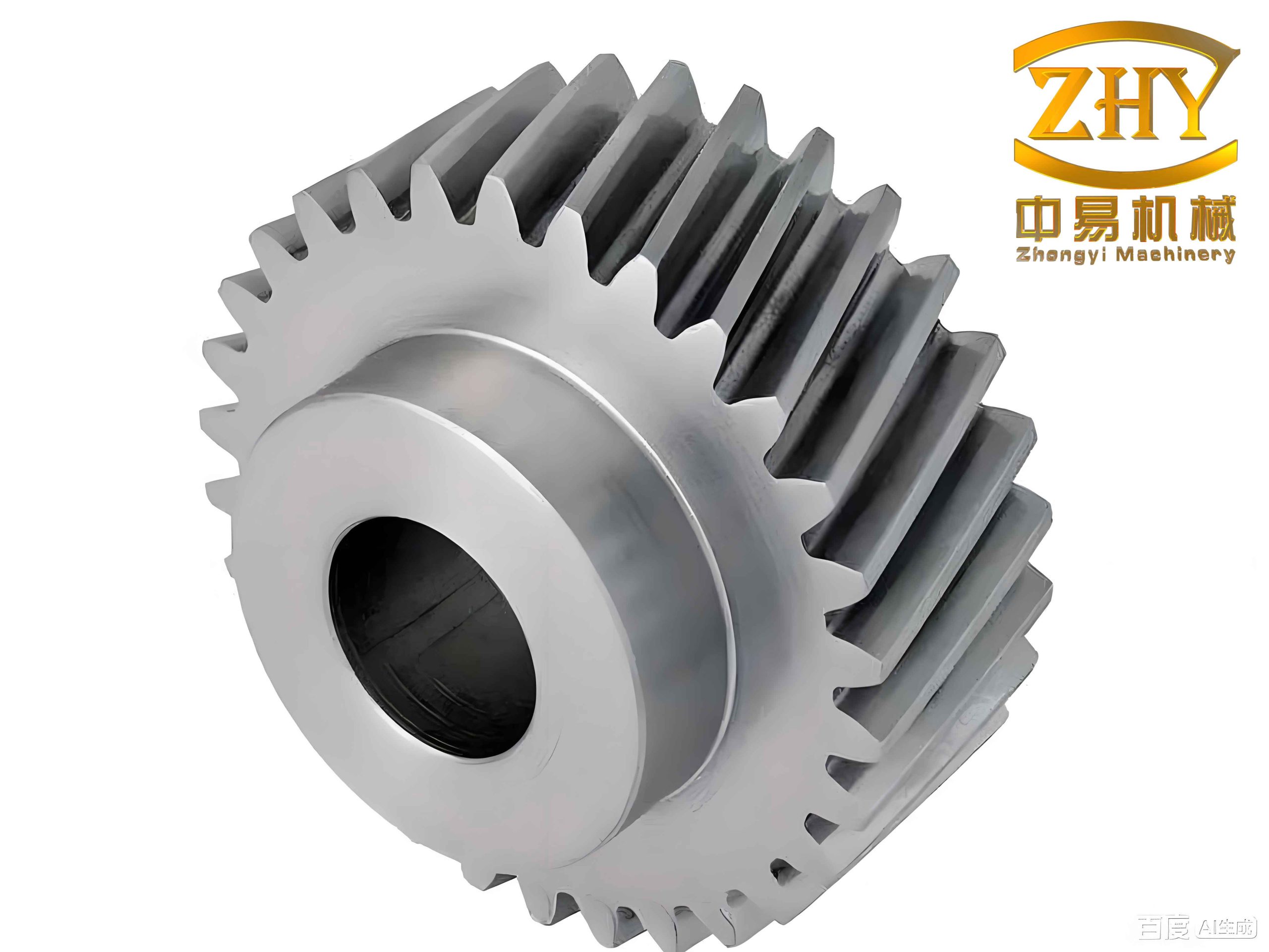
I begin from the observation that hydraulic systems in modern industrial equipment require compact pumps with high power density, low noise, and stable delivery. Helical gears are attractive in this context because their gradual tooth engagement distributes load over a longer contact line than spur gears. However, helical gears also introduce axial force components, coupled bending-torsional-axial motion, and additional thermal effects near the meshing zone. In a circular-arc helical gear pump, the fluid domain is bounded by rotating helical gears, stationary casing walls, inlet and outlet ports, and narrow leakage gaps. The temperature field changes oil viscosity, the pressure field changes the cavitation threshold, and the structural field deforms under pressure and thermal load. These effects feed back into vibration, sometimes in ways that are not obvious from a dry modal analysis. My purpose is therefore to formulate a coupled model, simulate the pump under realistic high-speed conditions, and confirm the predicted trends with vibration tests.
Why helical gears matter in this pump class
I treat helical gears not merely as transmission elements but as the main source of both positive displacement and dynamic excitation. The helical gears inside the pump trap oil between tooth spaces and the casing, carry it from the inlet side to the outlet side, and release it as the teeth remesh. Because the teeth are inclined, the contact line sweeps axially, and the meshing stiffness varies more smoothly than in a spur gear pump. This smooth variation is beneficial for noise, but it also creates axial vibration and a more complex force path through the bearings. In my model, the helical gears are represented with a six-degree-of-freedom generalized displacement vector:
$$ \{\delta\} = \{y_1, z_1, \theta_1, y_2, z_2, \theta_2\}^T $$
Here, \(y_i\) is the transverse vibration displacement along the line of action, \(z_i\) is the axial displacement, and \(\theta_i\) is the rotational displacement of rotor \(i\). The index \(i=1\) denotes the driving helical gear, and \(i=2\) denotes the driven helical gear. I write the dynamic equations of the helical gears as:
$$ m_1 \ddot{y}_1 + c_{1y}\dot{y}_1 + k_{1y}y_1 = -F_y $$
$$ m_1 \ddot{z}_1 + c_{1z}\dot{z}_1 + k_{1z}z_1 = -F_z $$
$$ I_1 \ddot{\theta}_1 = -F_y R_1 + T_1 + F_s(t)R_1 $$
$$ m_2 \ddot{y}_2 + c_{2y}\dot{y}_2 + k_{2y}y_2 = F_y $$
$$ m_2 \ddot{z}_2 + c_{2z}\dot{z}_2 + k_{2z}z_2 = -F_z $$
$$ I_2 \ddot{\theta}_2 = F_y R_2 – T_2 + F_s(t)R_2 $$
In these equations, \(m_i\) is rotor mass, \(I_i\) is rotary inertia, \(R_i\) is base circle radius, \(T_i\) is external torque, \(F_s(t)\) is the meshing impact force, \(F_y\) is the transverse dynamic meshing force, and \(F_z\) is the axial dynamic meshing force. For helical gears, the meshing force components can be expressed as:
$$ F_y = c_m \cos\beta\left(\dot{y}_1-\dot{y}_2+R_1\dot{\theta}_1-R_2\dot{\theta}_2\right) + k_m \cos\beta\left(y_1-y_2+R_1\theta_1-R_2\theta_2\right) $$
$$ F_z = c_m \sin\beta\left(\dot{z}_1-\dot{z}_2+\tan\beta(\dot{y}_1-\dot{y}_2+R_1\dot{\theta}_1-R_2\dot{\theta}_2)\right) + k_m \sin\beta\left(z_1-z_2+\tan\beta(y_1-y_2+R_1\theta_1-R_2\theta_2)\right) $$
where \(\beta\) is the helix angle, \(c_m\) is the normal meshing damping, and \(k_m\) is the normal meshing stiffness. This formulation shows why helical gears create coupled transverse-axial-rotational vibration. It also shows that increasing mass, stiffness, or damping can reduce the displacement under the same meshing force. I use this result later to guide structural optimization of the rotor.
Temperature rise and its mathematical control
I establish a temperature rise model because oil viscosity, density, and cavitation behavior all depend on temperature. The pump converts part of its mechanical energy into heat through viscous friction, pressure loss, and internal leakage. I start from mass conservation:
$$ \frac{dm}{dt} = \sum_i \dot{m}_i $$
The density of the oil changes with pressure and temperature:
$$ \frac{d\rho}{dt} = \left(\frac{\partial \rho}{\partial p}\right)_T \frac{dp}{dt} + \left(\frac{\partial \rho}{\partial T}\right)_p \frac{dT}{dt} $$
I introduce the isothermal bulk modulus and the isobaric thermal expansion coefficient:
$$ K_T = \rho\left(\frac{\partial p}{\partial \rho}\right)_T $$
$$ \alpha_p = -\frac{1}{\rho}\left(\frac{\partial \rho}{\partial T}\right)_p $$
Combining these relations with the volume change of a control volume gives the thermal pressure equation:
$$ \frac{dp}{dt} = \frac{K_T}{\rho}\left(\sum_i \dot{m}_i – \frac{\rho}{V}\frac{dV}{dt} – \alpha_p \frac{dT}{dt}\right) $$
This equation indicates that oil flow into a control volume raises pressure, volume expansion lowers pressure, and temperature rise modifies pressure through expansion. The energy conservation equation is:
$$ \frac{d}{dt}(mu) = Q – W + \sum_i \dot{H}_i $$
where \(Q\) is heat transfer rate, \(W\) is work done by the boundary, and \(\dot{H}_i\) is enthalpy flow rate. Using internal energy \(u = h – pV/m\), the differential enthalpy relation, and the boundary work \(p\,dV/dt\), I obtain the temperature rise control equation:
$$ \frac{dT}{dt} = \frac{1}{c_p V}\left[Q + \sum_i \dot{H}_i – \sum_i \dot{m}_i h_i + T V \alpha_p \frac{dp}{dt}\right] $$
From this equation I conclude three practical points. First, viscous friction inside the oil generates heat and raises the local temperature. Second, a pressure difference between regions changes the temperature through compression and expansion. Third, the specific enthalpy difference between the inlet and outlet fluids also changes the fluid temperature. These effects are important in high-speed helical gears because the meshing zone experiences rapid pressure changes, high shear rates, and repeated compression-expansion cycles.
Cavitation model and coupling with thermal effects
I use a full cavitation model because high-speed circular-arc helical gear pumps can develop low-pressure regions near the meshing zone, especially where the teeth separate and the chamber volume expands suddenly. The local pressure can drop below the vapor pressure of the oil, forming vapor bubbles. When these bubbles collapse, they generate local pressure impulses that excite vibration. I model the bubble dynamics with the Rayleigh-Plesset equation:
$$ \frac{p_B-p}{\rho_l} = r_B \frac{d^2 r_B}{dt^2} + \frac{3}{2}\left(\frac{dr_B}{dt}\right)^2 + \frac{4\nu_l}{r_B}\frac{dr_B}{dt} + \frac{2\sigma}{\rho_l r_B} $$
where \(r_B\) is bubble radius, \(p_B\) is pressure at the bubble wall, \(\rho_l\) is liquid density, \(\nu_l\) is kinematic viscosity, and \(\sigma\) is surface tension. I treat the mixture as a two-phase, three-component medium containing liquid oil, vapor, and non-condensable gas. The mixture density and viscosity are weighted by vapor volume fraction \(\phi_v\):
$$ \rho_m = \rho_v \phi_v + \rho_l(1-\phi_v) $$
$$ \mu_m = \mu_v \phi_v + \mu_l(1-\phi_v) $$
The vapor mass transfer rate is calculated from the simplified bubble dynamics. For the Zwart-Gerber-Belamri cavitation model, the net phase change rate \(R=R_e-R_c\) controls the vapor source term. I include the thermal effect by allowing the bubble growth rate to depend on temperature:
$$ \frac{dR}{dt} = f(p,p_B,T,T_\infty) $$
A higher local temperature increases the bubble growth rate, which lowers the cavitation vibration frequency. A lower local temperature accelerates bubble collapse, which raises the vibration frequency. The characteristic collapse time and frequency can be approximated as:
$$ T_c \approx 0.915 R_B \sqrt{\frac{\rho_l}{p_\infty}} $$
$$ f_c \approx \frac{1}{T_c} \approx \frac{1.093}{R_B}\sqrt{\frac{p_\infty}{\rho_l}} $$
These expressions are useful because they connect the thermal state to the frequency content of cavitation-induced vibration. In my numerical model, I activate the energy equation, viscous heating, and the RNG \(k-\varepsilon\) turbulence model so that swirl, jet impact, and local temperature rise are represented. The cavitation source term interacts with the temperature field, and the temperature field changes the oil viscosity and vapor pressure. This is the basis of my thermal-fluid-solid coupling approach.
Thermal-fluid-solid coupling formulation
I use a one-way loose coupling strategy for the pump because the structural deformation is small compared with the fluid domain size, although the temperature effect is important. I first solve the fluid domain to obtain pressure and temperature. Then I transfer the temperature to the solid domain for thermal analysis. Finally, I apply both the fluid pressure and the solid temperature to the structural model for coupled stress and modal analysis. The interface conditions are:
$$ \sigma_f \cdot n_f = \sigma_s \cdot n_s $$
$$ T_f = T_s $$
$$ q_f = q_s $$
$$ l_f = l_s $$
where \(\sigma\) is stress, \(T\) is temperature, \(q\) is heat flux, and \(l\) is displacement. The structural constitutive relation with thermal strain is:
$$ \sigma = D(\epsilon-\epsilon_0) $$
Here, \(D\) is the elasticity matrix, \(\epsilon\) is mechanical strain, and \(\epsilon_0\) is thermal strain. For isotropic material behavior:
$$ \epsilon_0 = \alpha \Delta T \{1,1,1,0,0,0\}^T $$
The finite element strain-displacement relation is:
$$ \epsilon = B\delta_e $$
and the thermal load vector is:
$$ Q_e = K\delta_e $$
For a material with thermal expansion, the total strain is written as:
$$ \epsilon = D^{-1}\sigma + \epsilon_{th} $$
$$ \epsilon_{th} = \{\alpha_x\Delta T,\alpha_y\Delta T,\alpha_z\Delta T,0,0,0\}^T $$
These equations form the thermal-fluid-solid coupling model that I use for the pump and rotor. The model is not just a thermal expansion calculation. It combines fluid pressure, temperature-dependent oil properties, cavitation, and structural deformation in a consistent sequence.
Pump geometry and simulation setup
I model a high-speed circular-arc helical gear pump with the following nominal parameters. The pump is designed for a load pressure of 25 MPa, a displacement of 5 mL/r, and a speed of 10000 r/min. The helical gears have seven teeth, module 3 mm, face width 15.5 mm, pressure angle 14.5°, and helix angle 31.3°. The center distance is 21.01 mm, and the shaft diameter in the baseline design is 10 mm. The inlet diameter is 16 mm, and the outlet diameter is 11 mm.
| Parameter | Value |
|---|---|
| Number of teeth | 7 |
| Module | 3 mm |
| Face width | 15.5 mm |
| Pressure angle | 14.5° |
| Helix angle | 31.3° |
| Center distance | 21.01 mm |
| Shaft diameter, baseline | 10 mm |
| Inlet diameter | 16 mm |
| Outlet diameter | 11 mm |
| Displacement | 5 mL/r |
| Rated speed | 10000 r/min |
| Load pressure | 25 MPa |
I build the fluid domain by Boolean subtraction of the solid helical gears from the pump casing volume. The fluid domain includes the inlet port, outlet port, tooth chambers, meshing clearance, and leakage paths. The meshing clearance is approximately 0.02 mm, so the mesh must be fine near the helical gears while remaining computationally efficient elsewhere. I use Hypermesh for the two-dimensional surface mesh and then convert it into a three-dimensional polyhedral mesh in Fluent Meshing. Polyhedral cells reduce cell count compared with tetrahedral meshes and usually improve convergence for rotating machinery.
The oil properties are listed below. I use Shell Tellus S2 M 22 hydraulic oil as the working fluid because its viscosity-temperature behavior is stable in high-pressure hydraulic systems.
| Property | Value |
|---|---|
| Density | 870 kg/m³ |
| Specific heat capacity | 1687 J/(kg·K) |
| Thermal conductivity | 0.12 W/(m·K) |
| Dynamic viscosity | 0.0225 kg/(m·s) |
I set the inlet pressure to 0.1 MPa and the outlet pressure to 25 MPa. The driving helical gear rotates clockwise, and the driven helical gear rotates counterclockwise. The user-defined function applies angular velocities of \(-1046\) rad/s and \(1046\) rad/s, which correspond to 10000 r/min. I use the pressure-based solver, unsteady flow, the RNG \(k-\varepsilon\) turbulence model, the energy equation, and viscous heating. The coupled pressure-velocity scheme is used with a least-squares cell-based gradient. I set pressure, momentum, and energy relaxation factors to 0.5 and keep other factors at default values.
Fluid domain results
I find that the pressure rises from the inlet to the outlet in a stepwise manner. The lowest pressure occurs at the inlet, and the highest pressure occurs at the outlet. In the meshing region, especially near the inlet side, there is a prominent negative pressure zone. As the helical gears rotate, each tooth chamber is isolated and transported toward the outlet. The pressure inside each chamber remains relatively uniform, but the chamber pressure increases as it approaches the outlet. This behavior confirms that the helical gears provide positive displacement and that the pressure difference is built across the meshing line. The pressure distribution also explains why the meshing zone is a critical region for both cavitation and vibration.
The temperature field shows that the inlet temperature is the lowest and the outlet temperature is slightly higher. The largest temperature rise occurs in the meshing region, particularly near the inlet side where the teeth separate. Along the tooth chambers from inlet to outlet, the temperature change is moderate. The overall temperature difference between inlet and outlet is not large, but the local hot spot in the meshing zone is important because it changes oil viscosity and cavitation behavior. I observe that the temperature rise is not uniform; it is concentrated where shear and pressure changes are strongest. This supports my decision to include temperature in the cavitation and structural models.
The cavitation field shows that vapor appears mainly on the side where the helical gears begin to separate. In that region, the chamber volume expands rapidly, the pressure drops, and the oil can vaporize. The high vapor volume fraction region is narrow but intense. This is the main cavitation source in the pump. Because the cavitation region is close to the meshing zone, its collapse impulses can directly excite the helical gears and the casing. The cavitation pattern also changes with speed and outlet pressure. At higher speed, the low-pressure region becomes more severe. At higher outlet pressure, the overall pressure level rises, but local low-pressure pockets can still form because of the rapid volume change.
Material and structural boundary conditions
I assign materials based on the function of each component. The driving and driven helical gears and shafts require high strength and wear resistance, so I use 20CrMnTi alloy steel. The front cover, rear cover, and pump body use ZL111 aluminum alloy to reduce weight while maintaining adequate stiffness. The sliding bearings use 7068 aluminum alloy because it has high yield strength and good thermal conductivity. Bolts use 35 carbon steel. Seals use nitrile rubber.
| Component | Material | Density (kg/m³) | Yield strength (MPa) | Thermal conductivity (W/(m·K)) |
|---|---|---|---|---|
| Driving and driven helical gears | 20CrMnTi | 7850 | 850 | 44.5 |
| Front and rear covers | ZL111 aluminum | 2700 | 260 | 130 |
| Pump body | ZL111 aluminum | 2700 | 260 | 130 |
| Sliding bearings | 7068 aluminum | 2850 | 603 | 140 |
| Bolts | 35 carbon steel | 7580 | 355 | 50 |
| Seals | Nitrile rubber | 1200 | — | 0.2 |
I apply bonded contact between the pump body and the covers because they are bolted together. I use frictionless contact between the two helical gears because an oil film separates them. I use frictional contact between the helical gear shafts and the sliding bearings with a low friction coefficient of 0.01 to represent the lubricating film. I apply bonded contact between the sliding bearings and the pump body because no relative sliding is expected. Bolts are preloaded with 100 N. The front cover includes an axial force balance groove that produces approximately 1133 N. The hydrostatic sliding bearings generate radial compensation forces of about 4957 N on the driving shaft and 6667 N on the driven shaft. I apply a motor torque of 10000 N·mm. These boundary conditions are summarized below.
| Boundary condition | Value |
|---|---|
| Fluid pressure load | From fluid simulation |
| Motor torque | 10000 N·mm |
| Driving shaft radial compensation | 4957 N |
| Driven shaft radial compensation | 6667 N |
| Driving shaft axial compensation | 1133 N |
| Bolt preload | 100 N |
| Bearing friction coefficient | 0.01 |
Static structural response and deformation
Under thermal-fluid-solid coupling at 10000 r/min and 25 MPa, the equivalent stress is concentrated at the sliding bearings and at the interface between the fluid and solid domains. The inlet region has an equivalent stress of about 55 MPa, and the outlet region has about 80 MPa. The contact between the sliding bearing and the driving helical gear shaft reaches about 236.1 MPa. The global maximum equivalent stress is 493.4 MPa at the contact between the sliding bearing and the driven helical gear shaft. Since the bearing material has a yield strength of 603 MPa, the maximum stress remains below the yield limit. I therefore conclude that the pump does not undergo plastic deformation under the rated thermal-fluid-solid coupling condition.
The deformation field shows that the front cover on the driving side experiences the largest displacement, reaching about 0.036 mm. This region is also close to the bearing support and the high-pressure outlet. The concentration of deformation suggests that the front cover is a preferred measurement point for vibration testing. The deformation is driven mainly by pressure and temperature, and it is not uniform across the casing. This is important because a casing deformation can change the clearance between the helical gears and the casing, which in turn changes leakage, cavitation, and vibration.
Dry and wet modal analysis of the pump
I perform dry modal analysis first to understand the structural stiffness distribution without fluid loading. The first two dry modes occur mainly in the keyway region of the driving shaft, which indicates that this region is vibration-sensitive. The third to sixth dry modes show significant vibration at the rounded corners of the rear cover. In the third mode, the diagonal rounded corners of the rear cover form two groups and oscillate in opposite axial directions. In the fourth mode, two opposite long-edge rounded corners oscillate together. In the fifth mode, all four rounded corners oscillate in phase along the axial direction. The sixth mode is similar to the fourth mode but with the two opposite short-edge rounded corners oscillating.
I then perform wet modal analysis under thermal-fluid-solid coupling. The first wet mode shows axial stretching of the front cover and pump body. The second and third wet modes show rocking of the front cover and pump body in planes perpendicular to the axis, with the two rocking directions perpendicular to each other. The fourth wet mode shows torsional vibration of the front cover and pump body in the plane perpendicular to the axis. The fifth and sixth wet modes show in-plane rocking around the center of the rear cover, again with a ninety-degree phase difference. Compared with the dry modes, the wet modes are shifted toward the pump body and rear cover edges because the wet model constrains the bolt holes and keyways. This constraint suppresses vibration in those regions and changes the mode shapes.
| Mode order | Dry natural frequency (Hz) | Wet natural frequency (Hz) | Change rate |
|---|---|---|---|
| 1 | 2686 | 1016 | 62.19% |
| 2 | 2705 | 1802 | 33.38% |
| 3 | 5802 | 2713 | 53.24% |
| 4 | 8371 | 5960 | 28.80% |
| 5 | 8480 | 6598 | 22.19% |
| 6 | 8774 | 7929 | 9.63% |
The wet natural frequencies are lower than the dry natural frequencies at every mode order. The first mode drops by 62.19%, and the third mode drops by 53.24%. As the mode order increases, the difference becomes smaller. This occurs because the fluid adds mass and damping to the system without adding much stiffness. The oil film and the surrounding fluid therefore reduce the natural frequencies and change the vibration response. I use these results to interpret the measured vibration spectra and to avoid resonance in the operating speed range.
Fatigue life and structural optimization
I evaluate fatigue life using the stress-life method and the Palmgren-Miner linear cumulative damage rule:
$$ D = \sum_i \frac{n_i}{N_i} $$
where \(D\) is cumulative damage, \(n_i\) is the actual number of cycles at stress level \(i\), and \(N_i\) is the allowable number of cycles at that stress level. Failure is predicted when \(D\) reaches unity. The baseline pump has a minimum fatigue life of \(1.8498\times10^{10}\) s at the interface between the driving shaft, sliding bearing, and pump body. At 10000 r/min, this corresponds to approximately 3.52 years of continuous operation, which satisfies the minimum three-year requirement. Other low-life regions include the driven shaft-sliding bearing contact and the rear cover bolt holes.
| Fatigue location | Fatigue life (s) | Fatigue damage |
|---|---|---|
| Driving shaft–sliding bearing | \(1.8479\times10^{10}\) | \(5.4061\times10^{-10}\) |
| Driven shaft–sliding bearing | \(2.5289\times10^{10}\) | \(3.9543\times10^{-10}\) |
| Rear cover bolt holes | \(3.1356\times10^{10}\) | \(3.1893\times10^{-10}\) |
Based on the theoretical result that rotor displacement under a given meshing force decreases with higher mass, stiffness, and damping, I optimize the rotor. I increase the driving and driven shaft diameters from 10 mm to 12 mm while keeping them smaller than the root circle diameter of the helical gears. This increases rotor mass and reduces the acceleration of vibration displacement. I also change the shaft material to 42CrMo alloy steel, which has higher stiffness and toughness. The optimization is intended to reduce vibration and improve fatigue life without sacrificing the positive displacement behavior of the helical gears.
| Metric | Baseline | Optimized | Improvement |
|---|---|---|---|
| Average flow rate | 45.7165 L/min | 45.8079 L/min | +0.2% |
| Flow pulsation rate | 22.65% | 17.69% | −28.05% |
| Volumetric efficiency | 91.42% | 91.62% | +0.2% |
| Minimum fatigue life | \(1.8498\times10^{10}\) s | \(1.9423\times10^{10}\) s | +4.8% |
| Estimated minimum service life | 3.52 years | 3.69 years | +4.8% |
The optimized pump maintains the same fatigue-critical regions, but the minimum life increases to \(1.9423\times10^{10}\) s. The average flow rate increases slightly, the flow pulsation decreases substantially, and the volumetric efficiency improves. I consider this a useful result because it shows that rotor stiffening and mass redistribution can reduce vibration while preserving or slightly improving hydraulic performance. The helical gears remain the main displacement elements, but their support structure becomes more resistant to dynamic deformation.
Rotor behavior under different coupling conditions
I analyze the rotor under four conditions: torque only, fluid-solid coupling, thermal-solid coupling, and thermal-fluid-solid coupling. The maximum deformation under torque only is about 0.001 mm, located at the keyway and the meshing region. Under fluid-solid coupling, the maximum deformation increases to about 0.0028 mm and is concentrated on the gear surfaces and the meshing point. Under thermal-solid coupling, the maximum deformation rises to about 0.0083 mm, with significant deformation at the tooth tips and the meshing region. Under thermal-fluid-solid coupling, the maximum deformation is about 0.0090 mm, again at the meshing region. The comparison shows that temperature has a stronger effect on rotor deformation than fluid pressure or torque alone. This is a key finding because it means that thermal effects cannot be neglected when predicting vibration in high-speed helical gears.
| Coupling condition | Maximum deformation (mm) | Dominant deformation region |
|---|---|---|
| Torque only | 0.001 | Keyway and meshing region |
| Fluid-solid | 0.0028 | Gear surfaces and meshing point |
| Thermal-solid | 0.0083 | Tooth tips and meshing region |
| Thermal-fluid-solid | 0.0090 | Meshing region and tooth tip clearance |
I compare the rotor modes without prestress and with thermal-fluid-solid coupling. Without prestress, the rotor modes are mainly bending and torsional vibration of the helical gears, with some combined modes. The first and third modes are bending along the \(x\)-axis, and the third mode has a larger bending amplitude. The second mode combines bending along the \(y\)-axis with torsion about the \(z\)-axis. The fourth mode combines bending along the \(x\)-axis with torsion about the \(y\)- and \(z\)-axes. The fifth mode combines bending along the \(x\)-axis with torsion about the \(x\)- and \(y\)-axes, and the two helical gears move in opposite directions. The sixth mode is mainly axial expansion along the \(z\)-axis.
Under thermal-fluid-solid coupling, the first rotor mode becomes axial expansion along the \(z\)-axis, with larger bending amplitude near the keyway. The second, third, and sixth modes are composite vibrations, and the amplitude is larger near the middle of the gear shaft. The second mode combines bending along the \(y\)-axis with torsion about the \(x\)-axis. The third mode combines torsion about the \(x\)-axis with torsion about the \(y\)-axis. The sixth mode combines bending along the \(y\)-axis with torsion about the \(x\)- and \(z\)-axes. The fourth and fifth modes are similar, both twisting about the \(z\)-axis, but the fourth has its largest bending amplitude along the \(x\)-axis, while the fifth has its largest bending amplitude along the \(y\)-axis. Overall, the thermal-fluid-solid coupling concentrates the rotor modes in the shaft region and increases the bending and twisting amplitudes compared with the no-prestress case.
| Mode order | No prestress (Hz) | Thermal-fluid-solid (Hz) | Change rate |
|---|---|---|---|
| 1 | 4344 | 1610 | 62.93% |
| 2 | 4502 | 2305 | 48.80% |
| 3 | 5639 | 2461 | 56.35% |
| 4 | 5650 | 4043 | 28.43% |
| 5 | 6061 | 4405 | 27.32% |
| 6 | 6450 | 4811 | 25.40% |
I calculate the critical speed from the first natural frequency:
$$ n = 60 f $$
Without prestress, the first critical speed is 260640 r/min. Under thermal-fluid-solid coupling, the first critical speed is 96600 r/min. The design speed is 10000 r/min, which is far below 0.6 times the coupled critical speed. The shaft frequency at 10000 r/min is 166.7 Hz, and the outlet pulsation frequency for seven teeth is about 1166.9 Hz. Both are well below the first coupled natural frequency of the rotor. Therefore, the rotor behaves as a rigid shaft in the intended operating range, and resonance is not expected at the rated speed. This result supports the design and provides a margin for speed variation.
Experimental platform and measurement plan
I build a vibration test platform for the high-speed circular-arc helical gear pump. The platform includes a hydraulic workstation and a dynamic signal acquisition system. The hydraulic workstation uses an 800 L stainless steel oil tank with suction and return filters, air filter, level gauge, pressure gauges, and hydraulic valves. The pump is connected to a servo motor through a diaphragm coupling. I install three acceleration sensors at the inlet port, the outlet port, and the front cover edge. I also install a temperature sensor at the front cover. The acceleration sensors are connected to a DH5902 dynamic signal acquisition system controlled by a host computer.
| Sensor | Model or type | Location or function |
|---|---|---|
| Acceleration sensor 1 | SN LW 204165 | Inlet port |
| Acceleration sensor 2 | SN LW 146976 | Front cover edge |
| Acceleration sensor 3 | SN LW 204182 | Outlet port |
| Turbine flow meter | LWY-WB15 | Return line |
| Pressure transmitter | TY-811-A1 | Return line |
The acceleration sensors have a sensitivity of about 10.18 mV/(m/s²), a measurement range of ±961 m/s², and a frequency response of 0.3–6 kHz. The turbine flow meter has a nominal diameter of DN15, a nominal pressure of 25 MPa, and a flow range of 0.6–6 m³/h. The pressure transmitter has a range of 0–40 MPa and an accuracy of ±0.2%. I test the pump at speeds of 4000, 6000, and 8000 r/min and outlet pressure loads of 0, 5, 10, and 15 MPa. I use a controlled-variable method so that the effects of speed and pressure load can be separated.
Signal processing with ICEEMDAN
I process the measured vibration signals with the improved complete ensemble empirical mode decomposition with adaptive noise, usually abbreviated as ICEEMDAN. This method is a development of empirical mode decomposition, ensemble empirical mode decomposition, and complete ensemble empirical mode decomposition. It reduces mode mixing and residual noise while preserving the local nonlinear and nonstationary features of the vibration signal. I use it because the vibration of helical gears contains meshing impacts, cavitation impulses, structural resonances, and fluid pressure pulsations that overlap in time and frequency.
The empirical mode decomposition residual relation is:
$$ r_k(t) = r_{k-1}(t) – IMF_k(t) $$
The ensemble empirical mode decomposition adds white noise realizations:
$$ x_i(t) = x(t) + w_i(t) $$
and averages the resulting intrinsic mode functions:
$$ IMF_k = \frac{1}{N}\sum_{i=1}^{N} IMF_k^{(i)} $$
The ICEEMDAN algorithm uses adaptive noise and local mean operators. I write the main steps as:
$$ x_i(t) = x(t) + \beta_0 E_1(w_i(t)) $$
$$ r_1 = \langle M(x_i(t)) \rangle $$
$$ IMF_1 = x(t) – r_1 $$
$$ r_k = \langle M(r_{k-1} + \beta_{k-1}E_k(w_i(t))) \rangle $$
$$ IMF_k = r_{k-1} – r_k $$
Here, \(E_k(\cdot)\) is the operator that extracts the \(k\)-th empirical mode, \(M(\cdot)\) produces the local mean, \(\beta\) controls the signal-to-noise ratio, and \(\langle \cdot \rangle\) denotes the ensemble average. I obtain six intrinsic mode functions and one residual for each measured signal. To select the most informative component, I calculate fuzzy entropy and kurtosis. Kurtosis is defined as:
$$ K_{ur} = \frac{\sum_i (IMF_i-\mu_i)^4}{\sigma_i^4} $$
where \(\mu_i\) is the mean and \(\sigma_i\) is the standard deviation of the \(i\)-th intrinsic mode function. A higher kurtosis indicates more impulsive content. Fuzzy entropy \(Y_{FE}\) measures signal uncertainty and correlation. I combine them into a comprehensive index:
$$ K = Y_{FE} + \frac{1}{K_{ur}} $$
A lower \(K\) value indicates that the intrinsic mode function is more sensitive to the original vibration signal and contains richer impact information. I calculate this index for the pump at 6000 r/min and 15 MPa. The results are shown below.
| IMF | Fuzzy entropy \(Y_{FE}\) | Kurtosis \(K_{ur}\) | Comprehensive index \(K\) |
|---|---|---|---|
| IMF1 | 4.1446 | 0.4742 | 6.2534 |
| IMF2 | 3.8272 | 0.3169 | 6.9828 |
| IMF3 | 5.3870 | 0.5209 | 7.3068 |
| IMF4 | 6.4688 | 0.6370 | 8.2187 |
| IMF5 | 6.1537 | 0.4969 | 8.1662 |
| IMF6 | 3.5575 | 0.1190 | 11.9609 |
| Residual | 2.1096 | 0.0023 | 436.89 |
IMF1 has the smallest comprehensive index, so I select IMF1 as the main component for vibration characteristic analysis. Its dominant frequency band is close to that of the original signal, which confirms that it captures the most relevant dynamic information. I therefore use IMF1 in the subsequent comparisons of position, speed, and pressure load.
Vibration differences at different pump locations
I compare the vibration amplitudes at the inlet port, outlet port, and front cover edge. At 4000 r/min and 0 MPa, the vibration curves at the three locations are relatively smooth and the amplitudes are small. The inlet, outlet, and cover signals are similar, which suggests that the pump behaves in a relatively uniform way at low speed and low load. At 6000 r/min and 0 MPa, and at 8000 r/min and 0 MPa, the vibration amplitude and fluctuation increase. This is a direct consequence of higher rotational speed and stronger meshing excitation. Under 0 MPa, the outlet port generally has a larger vibration amplitude than the inlet port and the front cover edge. The inlet port and front cover edge have similar amplitudes. Under 15 MPa, however, the front cover edge can slightly exceed the inlet port. This shows that pressure load changes the distribution of vibration among the pump locations.
| Condition | Inlet port | Outlet port | Front cover edge |
|---|---|---|---|
| 4000 r/min, 0 MPa | Low and smooth | Low and smooth | Low and smooth |
| 6000 r/min, 0 MPa | Moderate | Higher | Moderate |
| 8000 r/min, 0 MPa | Moderate | Highest | Moderate |
| 8000 r/min, 15 MPa | Moderate | High | Slightly higher than inlet |
The outlet port is a key location because it combines internal fluid dynamic effects with the external connection to the hydraulic circuit. The front cover edge is also important because the static analysis shows the largest deformation there. I therefore focus the detailed speed and pressure analyses on the outlet region and use the other locations to confirm the spatial distribution.
Effect of rotational speed on vibration
I analyze the IMF1 time-domain and frequency-domain results at 0 MPa and 15 MPa for speeds of 4000, 6000, and 8000 r/min. At 0 MPa, the vibration amplitude increases with speed. At 4000 r/min, the amplitude is about 2.63 m/s². At 6000 r/min, it rises to about 5.26 m/s². At 8000 r/min, it increases sharply to about 11.36 m/s². At 15 MPa, the same increasing trend appears, but the growth is more pronounced. This means that speed and pressure load have a combined effect: higher pressure makes the pump more sensitive to speed-induced vibration.
| Pressure load | Speed | Amplitude trend | Peak frequency and amplitude |
|---|---|---|---|
| 0 MPa | 4000 r/min | About 2.63 m/s² | Peak A: 642.9 Hz, 0.23 |
| 0 MPa | 6000 r/min | About 5.26 m/s² | Peak B: 651.3 Hz, 0.23 |
| 0 MPa | 8000 r/min | About 11.36 m/s² | Peak C: 683.7 Hz, 0.67 |
| 15 MPa | 4000 r/min | Lower than 8000 r/min | Peak D: 634.8 Hz, 0.17 |
| 15 MPa | 6000 r/min | Intermediate | Peak E: 634.8 Hz, 0.51 |
| 15 MPa | 8000 r/min | Highest | Peak F: 634.8 Hz, 1.07 |
In the frequency domain at 0 MPa, the main peak frequency increases slightly with speed. The peak amplitudes at 4000 and 6000 r/min are similar, but the 8000 r/min peak is about 2.9 times larger. At 15 MPa, the peak frequency remains nearly constant, but the amplitude increases with speed. This indicates that pressure load can lock the dominant frequency to a certain band while increasing its energy. The frequency band of interest is roughly 500–800 Hz, which is below the coupled natural frequencies of the pump and rotor. Therefore, the measured vibration is not a direct resonance of the first coupled mode but is driven by meshing, cavitation, and flow pulsation.
Effect of pressure load on vibration
I analyze the IMF1 results at 6000 and 8000 r/min for pressure loads of 0, 5, 10, and 15 MPa. At 6000 r/min, the overall vibration amplitude increases with pressure load, but there is a slight decrease at 10 MPa. At 8000 r/min, the amplitude increases from 0 to 10 MPa and then decreases at 15 MPa. This means that the pressure load at which the vibration drops depends on speed. The frequency-domain results support this observation. At 6000 r/min, the main peaks are G, H, I, and J. Peak G at 0 MPa is 667.5 Hz with amplitude 0.47. Peak H at 5 MPa is 667.5 Hz with amplitude 0.91. Peak I at 10 MPa is 618.8 Hz with amplitude 0.84. Peak J at 15 MPa is 683.7 Hz with amplitude 1.30. At 8000 r/min, peak K at 0 MPa is 683.7 Hz with amplitude 0.68. Peak L at 5 MPa is 634.8 Hz with amplitude 1.12. Peak M at 10 MPa is 634.8 Hz with amplitude 1.29. Peak N at 15 MPa is 683.7 Hz with amplitude 1.01.
| Speed | Pressure load | Peak label | Frequency (Hz) | Amplitude |
|---|---|---|---|---|
| 6000 r/min | 0 MPa | G | 667.5 | 0.47 |
| 6000 r/min | 5 MPa | H | 667.5 | 0.91 |
| 6000 r/min | 10 MPa | I | 618.8 | 0.84 |
| 6000 r/min | 15 MPa | J | 683.7 | 1.30 |
| 8000 r/min | 0 MPa | K | 683.7 | 0.68 |
| 8000 r/min | 5 MPa | L | 634.8 | 1.12 |
| 8000 r/min | 10 MPa | M | 634.8 | 1.29 |
| 8000 r/min | 15 MPa | N | 683.7 | 1.01 |
I interpret the non-monotonic behavior as follows. As pressure load increases, the pump must work against a higher outlet pressure, so the meshing force and bearing load generally increase. However, the higher pressure also suppresses cavitation in some regions and changes the oil film stiffness and damping. At a certain combination of speed and pressure, the cavitation intensity may decrease, or the fluid film may become more stable, which reduces the measured vibration. This is why the vibration amplitude can drop at a specific pressure load. The drop point is not fixed; it moves with speed. I consider this an important result for condition monitoring because it means that a lower vibration amplitude does not always mean a lower load or a safer condition.
RMS vibration energy comparison
I compute the root mean square value of the IMF1 component to quantify vibration energy:
$$ RMS = \sqrt{\frac{1}{n}\sum_{i=1}^{n} x_i^2} $$
The RMS value increases with speed at constant pressure. At 0, 5, and 10 MPa, the RMS increases slightly from 4000 to 6000 r/min and then increases significantly from 6000 to 8000 r/min. At 15 MPa, the trend is different: the RMS increases greatly from 4000 to 6000 r/min but the increase from 6000 to 8000 r/min is smaller. At constant speed, the RMS generally rises with pressure load, but there are local drops. At 4000 and 6000 r/min, the RMS rises from 0 to 5 MPa, decreases from 5 to 10 MPa, and rises again at 15 MPa. At 8000 r/min, the RMS rises from 0 to 10 MPa and then decreases at 15 MPa. These RMS trends match the time-domain and frequency-domain observations.
| Speed | 0 MPa | 5 MPa | 10 MPa | 15 MPa |
|---|---|---|---|---|
| 4000 r/min | Lowest | Slight rise | Slight drop | Rise again |
| 6000 r/min | Low | Rise | Drop | Rise |
| 8000 r/min | Moderate | Higher | Highest | Drop |
The RMS analysis confirms that the vibration energy of the pump is controlled by both speed and pressure load. Speed generally increases vibration energy because it increases meshing frequency, cavitation intensity, and flow pulsation. Pressure load increases the static and dynamic loads, but it also changes cavitation and film behavior. The combined effect is not monotonic at all operating points. This is why I use a coupled thermal-fluid-solid model and an experimental design with both variables rather than a single-variable correlation.
Interpretation through helical gears and coupled mechanisms
I return to the central role of helical gears in the observed vibration. The helical gears generate a time-varying meshing stiffness because the contact line length changes as the teeth roll. The axial contact ratio is greater than one, so the load transfer is smoother than in spur gears, but the axial force component still exists. The meshing force can be decomposed into transverse and axial components, and the axial component excites the shaft and bearing system. Temperature changes the tooth profile through thermal expansion, which reduces the backlash and increases the contact area. This increases the meshing stiffness and reduces the displacement under the same force. The same temperature rise reduces oil viscosity, which can increase leakage and change the cavitation threshold. Cavitation generates impulsive pressures when bubbles collapse, and those impulses are transmitted through the oil and the helical gears to the casing. The casing deformation then changes the clearance around the helical gears, which feeds back into leakage and cavitation. This chain of interactions explains why the measured vibration is sensitive to speed and pressure load and why a purely structural modal analysis is insufficient.
I also note that the rotor optimization works because it changes the mass, stiffness, and damping of the helical gear rotor system. Increasing the shaft diameter from 10 mm to 12 mm increases the second moment of area and the mass. The higher stiffness reduces the displacement under the meshing force. The higher mass reduces the acceleration for the same force, as shown by:
$$ F = m\ddot{x} + c\dot{x} + kx $$
and the steady-state amplitude under harmonic excitation is:
$$ X = \frac{F_0}{\sqrt{(k-m\omega^2)^2 + (c\omega)^2}} $$
These relations show that increasing \(k\) and \(c\) reduces amplitude, while increasing \(m\) shifts the resonance frequency. The material change to 42CrMo further increases strength and fatigue resistance. The result is a small improvement in flow and volumetric efficiency, a significant reduction in flow pulsation, and a longer fatigue life. This is consistent with my theoretical prediction that the helical gears and their support structure should be treated as a coupled dynamic system.
Summary of numerical and experimental trends
I summarize the main trends in the following table. The numerical simulations show that pressure, temperature, and cavitation are concentrated near the meshing zone of the helical gears. The static analysis shows that the maximum equivalent stress remains below the yield strength. The modal analysis shows that the wet natural frequencies are much lower than the dry natural frequencies. The fatigue analysis shows that the minimum life is at the bearing-shaft interface and that the optimized design improves life by about 4.8%. The experiments show that the outlet port generally has the highest vibration, that vibration increases with speed, and that pressure load has a non-monotonic effect with a speed-dependent drop point.
| Observation | Numerical result | Experimental result |
|---|---|---|
| Pressure distribution | Stepwise rise from inlet to outlet; low pressure at meshing separation | Outlet vibration generally highest |
| Temperature distribution | Hot spot in meshing zone | Temperature affects oil viscosity and vibration |
| Cavitation | Strong vapor region near meshing separation | Vibration peaks in 500–800 Hz band |
| Speed effect | Higher speed increases cavitation and load fluctuation | Amplitude and RMS increase with speed |
| Pressure effect | Higher pressure increases load but can suppress cavitation | Non-monotonic amplitude with local drop |
| Critical speed | 96600 r/min under coupling | Operating speed 10000 r/min is safe |
| Fatigue life | Minimum 3.52 years baseline; 3.69 years optimized | No failure observed in test range |
Conclusions from my study
I have established a thermal-fluid-solid coupling framework for high-speed circular-arc helical gear pumps. The framework includes a temperature rise control equation, a full cavitation model, a coupled structural formulation, and a meshing vibration model for helical gears. I used the model to simulate the pump at 10000 r/min and 25 MPa, and I validated the main trends with a vibration test platform. The results show the following.
First, the pressure field rises from the inlet to the outlet, and the lowest pressure occurs near the meshing separation zone. The temperature rise is concentrated in the meshing region, where shear and pressure changes are strongest. Cavitation also occurs mainly near the meshing separation side. These three fields are spatially coupled, and their concentration near the helical gears explains why the meshing zone is the dominant vibration source.
Second, the static structural analysis shows that the maximum equivalent stress is 493.4 MPa, which is below the yield strength of the bearing material. The maximum deformation is about 0.036 mm at the front cover on the driving side. The dry and wet modal analyses show that the fluid reduces the natural frequencies, especially the first mode, by more than 60%. The fatigue analysis shows a minimum life of about 3.52 years for the baseline design, which satisfies the three-year requirement.
Third, the rotor analysis under torque, fluid-solid, thermal-solid, and thermal-fluid-solid conditions shows that temperature has the strongest effect on rotor deformation. The maximum deformation increases from 0.001 mm under torque only to 0.0090 mm under thermal-fluid-solid coupling. The coupled critical speed is 96600 r/min, which is much higher than the design speed of 10000 r/min. Therefore, the rotor is rigid in the operating range and resonance is not expected.
Fourth, the structural optimization increases the shaft diameter and changes the material to 42CrMo. The average flow rate increases slightly, the flow pulsation decreases by about 28.05%, the volumetric efficiency improves slightly, and the minimum fatigue life increases by about 4.8%. This confirms that reducing rotor vibration through mass, stiffness, and damping modification is compatible with hydraulic performance.
Fifth, the vibration experiments show that the outlet port has the highest vibration amplitude in most operating conditions. The vibration amplitude increases with speed, and the rate of increase becomes larger under higher pressure load. At constant speed, the vibration amplitude generally rises with pressure load but can drop at a specific pressure load. The drop point depends on speed, which suggests that cavitation suppression and oil film stabilization compete with the increased load. The RMS results confirm the same trend.
Sixth, the ICEEMDAN algorithm with fuzzy entropy and kurtosis is effective for extracting the most informative intrinsic mode function from the vibration signal. IMF1 has the lowest comprehensive index and the closest frequency band to the original signal, so it is suitable for analyzing the effects of speed and pressure load. This signal processing method helps separate the meshing and cavitation contributions from the overall vibration response.
Future work
I see several directions for further work. The present coupling is one-way loose coupling, so the fluid field does not receive feedback from structural deformation. A two-way thermal-fluid-solid coupling model would be more accurate if the clearance changes become large. I also did not obtain rated-condition vibration data for the prototype, so a direct comparison between simulation and experiment at the full design point remains to be done. In addition, the helical gears could be studied with different helix angles, tooth profiles, and surface treatments to see how the meshing stiffness and cavitation behavior change. A more detailed thermal model could include the temperature dependence of viscosity and vapor pressure in a transient form. Finally, the vibration signal could be combined with pressure and temperature signals for real-time condition monitoring, so that the speed-dependent pressure drop point can be identified online. These steps would strengthen the design of high-speed circular-arc helical gear pumps and improve their reliability in high-pressure hydraulic systems.