
1. Introduction and Research Context
Wind energy has become one of the most important renewable energy sources in the global transition toward cleaner power generation. According to the Global Wind Report 2023, the worldwide installed wind capacity has been growing steadily, with China contributing a significant share of the newly added capacity. Wind turbines operate under highly variable and demanding conditions, especially in large-scale installations located in remote areas such as highland plateaus and offshore regions. The gearbox, as the core component of a wind turbine drive train, directly affects the reliability, maintenance cost, and service life of the entire system. High-speed and heavy-load applications often adopt herringbone gears due to their superior load-carrying capacity, better meshing stability, and lower vibration levels compared with spur or helical gears.
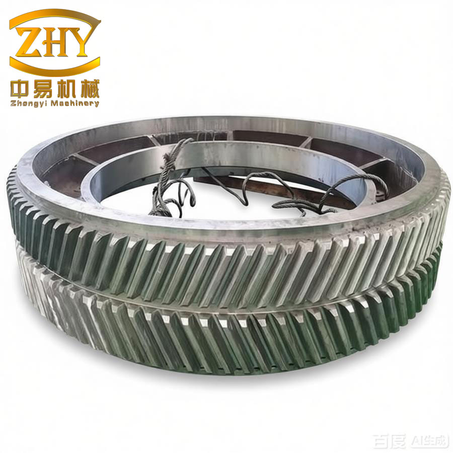
The herringbone gear is essentially composed of two oppositely inclined helical gear halves. This configuration eliminates axial thrust forces, making it particularly suitable for high-power transmission systems. However, under high rotational speeds and large torques, the frictional heat generated at the tooth contact surfaces causes a significant temperature rise in the gear body. The resulting thermal deformation, combined with mechanical elastic deformation, can lead to tooth profile deviations from the ideal conjugate geometry, increasing the risk of impact loads, noise, and premature failure modes such as scuffing and pitting.
The main objective of this thesis is to investigate the thermal-mechanical coupling behavior of a high-speed herringbone gear pair in a wind turbine gearbox and to propose a tooth profile modification method based on the coupled deformation. The research includes accurate parametric modeling of herringbone gears, calculation of frictional heat flux and convective heat transfer coefficients, finite element simulation of the steady-state temperature field, sequential thermal-mechanical coupling analysis, and finally the determination of optimal profile modification parameters. The results provide a theoretical basis for improving the performance and reliability of high-speed herringbone gear drives.
2. Basic Principles of Tooth Profile Modification and Parametric Modeling
2.1 Meshing Impact Mechanism
During gear operation, the actual meshing process differs from the ideal conjugate motion. The elastic deformation of gear teeth under load, thermal deformation caused by temperature rise, manufacturing errors, and assembly errors all contribute to a deviation from the theoretical meshing line. When the actual base pitch of a gear pair is not equal, the engagement begins earlier or ends later than the theoretical instant, producing an impact known as meshing-in shock or meshing-out shock. This impact generates additional dynamic loads, vibration, and noise.
For a pair of gears, when the driven gear tooth enters meshing at the tip circle, the load is normally carried by the preceding tooth pair. However, due to tooth deflection, the actual normal base pitch of the driven gear becomes larger than that of the driving gear, forcing the tooth pair to enter meshing prematurely. The instantaneous transmission ratio becomes:
$$ i_{12} = \frac{r_2 – \Delta r}{r_1 + \Delta r} < \frac{r_2}{r_1} $$
Similarly, when the driving gear tooth leaves meshing at its tip circle, the driven gear tooth pair tends to remain in contact longer than the theoretical period, resulting in a meshing-out shock. The instantaneous transmission ratio in this case is:
$$ i_{12} = \frac{r_2 + \Delta r’}{r_1 – \Delta r’} > \frac{r_2}{r_1} $$
To reduce these impacts, tooth profile modification is widely employed. By deliberately removing a small amount of material from the tooth tip or root, the actual contact path can be made closer to the ideal one under loaded conditions, thus smoothing the transition between single- and double-pair meshing zones.
2.2 Parameters of Tooth Profile Modification
Three fundamental parameters define a tooth profile modification: the maximum modification amount $\Delta_{\max}$, the modification length $l$, and the modification curve shape. Several empirical formulas have been proposed in the literature to determine the maximum modification amount.
The ideal maximum modification amount can be expressed as:
$$ \Delta_{\max} = \delta + \delta_{\theta} + \delta_m $$
where $\delta$ is the elastic deformation under load, $\delta_{\theta}$ is the thermal deformation due to temperature difference, and $\delta_m$ is the manufacturing error. The ISO standard recommends the following formula:
$$ \Delta_{\max} = \frac{K_A F_t / b}{C_r \varepsilon_{\alpha}} $$
where $K_A$ is the application factor, $F_t$ is the tangential force, $b$ is the face width, $C_r$ is the mesh stiffness, and $\varepsilon_{\alpha}$ is the transverse contact ratio.
The modification length is often selected according to empirical formulas. The ISO recommendation gives:
$$ L = 0.6 m_n $$
while other researchers suggest values between $0.5 m_n$ and $0.65 m_n$. For high-speed and heavy-load gears, long modification (extending from the mesh endpoint to the alternation point) is preferred.
The modification curve is described by the general power function:
$$ \Delta(x) = \Delta_{\max} \left( \frac{x}{L} \right)^p $$
where $x$ is the distance from the start of modification, and $p$ is the exponent. Common values of $p$ include $p=1$ (linear modification), $p=1.22$ (Hidaka-Terauchi), $p=1.5$ (Walker), and $p=1.43$ or $p=1.76$ (Li & Li). Another popular curve is the Minagawa-type profile given by:
$$ \Delta(x) = \Delta_{\max} \left[ 0.44 \left( \frac{x}{L} \right) + 0.56 \left( \frac{x}{L} \right)^2 \right] $$
2.3 Parametric Modeling of Herringbone Gear
An accurate three-dimensional model is essential for reliable finite element analysis. In this work, the gear tooth profile is generated by simulating the generation cutting process with a rack-type cutter. The coordinate transformation method is employed to derive the exact equations of the involute profile and the trochoidal root fillet.
Let the rack cutter be rigidly attached to a moving coordinate system, while the gear blank rotates about its center. A point on the cutter tooth profile with coordinates $(x_0,y_0)$ in the cutter frame can be transformed to the gear blank frame using the following transformation:
$$ \begin{cases} x = r(\varphi – \sin\varphi) + x_0 \cos\varphi – y_0 \sin\varphi \\ y = r(1 – \cos\varphi) + x_0 \sin\varphi + y_0 \cos\varphi \end{cases} $$
where $r$ is the pitch circle radius and $\varphi$ is the roll angle.
The root transition curve is generated by the cutter tip radius. For a point on the cutter tip arc with radius $\rho_0$ and center at $(x_c, y_c)$, the coordinates in the cutter frame are:
$$ \begin{cases} x_0 = x_c + \rho_0 \cos\gamma \\ y_0 = y_c – \rho_0 \sin\gamma \end{cases} $$
where $\gamma$ defines the angular position on the tip arc. Substituting these expressions into the transformation equation gives the transition curve.
The involute profile is produced by the straight-line portion of the rack cutter. The resulting involute curve in the gear frame can be written as:
$$ \begin{cases} x = \left[ r – \left( \frac{1}{2} \pi m + x_w \right) \sin\alpha \right] \cos\varphi + \left[ r – \left( \frac{1}{2} \pi m + x_w \right) \sin\alpha \right] \sin\varphi \\ y = \left[ r – \left( \frac{1}{2} \pi m + x_w \right) \sin\alpha \right] \sin\varphi – \left[ r – \left( \frac{1}{2} \pi m + x_w \right) \sin\alpha \right] \cos\varphi \end{cases} $$
where $x_w$ is the addendum modification coefficient, and $\alpha$ is the pressure angle.
Since the herringbone gear is a combination of two helical gears with opposite helix angles, the three-dimensional tooth surface equation is obtained by translating the end-section profile along a helix. The resulting surface coordinates are:
$$ \begin{cases} X = r \cos\left( \theta + \frac{Z}{r} \tan\beta \right) \\ Y = r \sin\left( \theta + \frac{Z}{r} \tan\beta \right) \\ Z = B t \end{cases} $$
where $\beta$ is the helix angle, $B$ is the face width, and $t \in [0,1]$ is a dimensionless parameter along the face width. For the mirrored half, the $Z$ coordinate is reversed.
The parametric modeling procedure consists of the following steps:
- Calculate the discrete points of the involute, transition curve, and tip circle using MATLAB.
- Import the point clouds into SolidWorks and fit them with spline curves to obtain the exact end-section tooth profile.
- Extrude the profile along the helix direction to create one helical half.
- Mirror the half about the midsection plane to create the herringbone gear.
- Assemble the driving and driven gears with the correct center distance.
Table 1 lists the main parameters of the herringbone gear pair studied in this thesis.
| Parameter | Symbol | Driving gear Z1 | Driven gear Z2 |
|---|---|---|---|
| Number of teeth | $Z$ | 31 | 102 |
| Normal module (mm) | $m_n$ | 4.5 | 4.5 |
| Normal pressure angle (°) | $\alpha_n$ | 20 | 20 |
| Helix angle (°) | $\beta$ | 25 | 25 |
| Face width (mm) | $B$ | 45 | 45 |
| Gap width (mm) | $B_1$ | 10 | 10 |
| Addendum modification coefficient | $x$ | 0 | 0 |
| Input torque (Nm) | $T_1$ | 4000 | – |
| Rotational speed (r/min) | $n$ | 5000 | 1519.6 |
3. Dynamic Contact and Thermal Analysis of High-Speed Herringbone Gear
3.1 Relative Sliding Velocity and Contact Pressure
During gear meshing, the sliding velocity at a given contact point $k$ along the line of action can be expressed as:
$$ V_{g} = V_{k1} – V_{k2} = \omega_1 \rho_{k1} – \omega_2 \rho_{k2} $$
where $\omega_1$ and $\omega_2$ are the angular velocities of the two gears, and $\rho_{k1}$, $\rho_{k2}$ are the radii of curvature at the contact point. The radii of curvature for an involute profile are:
$$ \rho_{k1} = \frac{r_{b1} \tan\alpha_{k1}}{\cos\beta_b}, \quad \rho_{k2} = \frac{r_{b2} \tan\alpha_{k2}}{\cos\beta_b} $$
where $r_{b1}$ and $r_{b2}$ are the base circle radii, $\alpha_{k1}$ and $\alpha_{k2}$ are the pressure angles at the point, and $\beta_b$ is the base helix angle.
The relative sliding velocity is zero at the pitch point and reaches its maximum near the tooth tip and tooth root. This variation directly affects the frictional heat generation along the tooth profile.
The contact pressure along the instantaneous contact line is calculated using Hertzian theory. For a helical gear, the contact can be approximated by slicing the tooth into a series of spur gear sections. The mean contact pressure at point $k$ is:
$$ p_k = \sqrt{ \frac{w_k E^*}{2\pi \rho_{k12}} } $$
where $w_k$ is the load per unit contact length, $E^*$ is the equivalent elastic modulus, and $\rho_{k12}$ is the equivalent radius of curvature:
$$ \rho_{k12} = \frac{\rho_{k1} \rho_{k2}}{\rho_{k1} + \rho_{k2}} $$
For the analyzed gear pair, the contact pressure and sliding velocity are computed at discrete positions along the meshing line. The results show that the sliding velocity has a maximum at the tooth root and tip regions, while the contact pressure exhibits a sharp increase at the transition points between single-pair and double-pair meshing zones.
3.2 Frictional Heat Flux
The instantaneous frictional heat flux generated at the contact point is given by:
$$ q_k = \gamma f p_k V_g $$
where $\gamma$ is the fraction of frictional energy converted into heat (taken as 0.95 in this study), and $f$ is the coefficient of friction. The friction coefficient is estimated from the empirical formula:
$$ f = 0.12 \left( \frac{w_k R_a}{\eta_f V_g \rho_{k12}} \right)^{0.25} $$
where $R_a$ is the average surface roughness, and $\eta_f$ is the dynamic viscosity of the lubricant.
The heat generated is distributed between the two gear bodies according to a partition coefficient $\beta$:
$$ \beta = \frac{\lambda_1 \sqrt{c_1 \rho_1 V_1}}{\lambda_1 \sqrt{c_1 \rho_1 V_1} + \lambda_2 \sqrt{c_2 \rho_2 V_2}} $$
where $\lambda$, $c$, and $\rho$ are the thermal conductivity, specific heat capacity, and density of each gear material, respectively. The heat flux allocated to the driving and driven gears is:
$$ q_{k1} = \beta q_k, \quad q_{k2} = (1-\beta) q_k $$
Because the contact time during one revolution is very short, the instantaneous heat flux is averaged over the full rotation period. The average heat flux for gear 1 at point $k$ is:
$$ Q_{k1} = q_{k1} \frac{2a}{V_{k1}} \cdot \frac{n_1}{60} $$
where $2a$ is the Hertzian contact width and $n_1$ is the rotational speed. The computed average heat flux distribution along the tooth profile is shown in Table 2 for several representative positions.
| Position on tooth profile | Sliding velocity (m/s) | Contact pressure (MPa) | Average heat flux of Z1 (W/mm²) | Average heat flux of Z2 (W/mm²) |
|---|---|---|---|---|
| Tooth root | 8.42 | 612.3 | 0.0921 | 0.0847 |
| Lower transition | 5.12 | 568.7 | 0.0612 | 0.0563 |
| Pitch point | 0 | 532.1 | 0 | 0 |
| Upper transition | 4.89 | 571.4 | 0.0588 | 0.0541 |
| Tooth tip | 7.94 | 620.5 | 0.0876 | 0.0805 |
3.3 Convective Heat Transfer Coefficients
The heat dissipation from the gear to the surrounding lubricant or air is governed by convective heat transfer. Different surfaces of the gear experience different flow conditions, so their heat transfer coefficients are calculated separately.
For the gear end face, the flow can be modeled as a rotating disk. The Reynolds number is:
$$ Re = \frac{\omega r^2}{\nu_f} $$
where $\omega$ is the angular velocity, $r$ is the radius, and $\nu_f$ is the kinematic viscosity of the lubricant. For the laminar flow regime ($Re < 2 \times 10^5$), the convective heat transfer coefficient is:
$$ \alpha_s = 0.308 (m+2)^{0.5} \lambda_f \left( \frac{\omega}{\nu_f} \right)^{0.5} Pr^{0.5} $$
Here, $m=2$ and $Pr$ is the Prandtl number. For the tooth face, the heat transfer coefficient varies along the tooth height and is expressed as:
$$ \alpha_s = \sqrt{ \frac{2 \omega}{\nu_f} } \lambda_f \left( \frac{C_f q_t Q}{\alpha H_c} \right)^{0.25} \left( \frac{H_c}{r} \right) $$
where $Q$ is the volumetric flow rate of the lubricant, $H_c$ is the local tooth height, and $\alpha$ is the thermal diffusivity of the lubricant.
For the tooth tip, the flow is approximated as a fluid over a flat plate:
$$ \alpha_s = 0.664 \lambda_f \left( \frac{\omega}{\pi \nu_f} \right)^{0.5} Pr^{1/3} $$
The calculated heat transfer coefficients for the driving and driven gears at the operating speed are summarized in Table 3.
| Surface | Heat transfer coefficient for Z1 (W/m²·K) | Heat transfer coefficient for Z2 (W/m²·K) |
|---|---|---|
| End face | 412.5 | 326.8 |
| Tooth face (root to tip) | 518.2 – 742.6 | 429.7 – 615.3 |
| Tooth tip | 377.4 | 302.1 |
The results show that the turbulent flow condition does not occur at the considered speeds. The heat transfer coefficients increase with rotational speed and are higher for the driving gear due to its smaller radius and higher angular velocity.
4. Thermal Analysis of Herringbone Gear Body
4.1 Heat Balance Equation
The temperature field inside the gear body satisfies the three-dimensional heat conduction equation:
$$ k \left( \frac{\partial^2 T}{\partial x^2} + \frac{\partial^2 T}{\partial y^2} + \frac{\partial^2 T}{\partial z^2} \right) = \rho c \frac{\partial T}{\partial t} $$
For steady-state operation, the temperature no longer changes with time, so the equation reduces to:
$$ \frac{\partial^2 T}{\partial x^2} + \frac{\partial^2 T}{\partial y^2} + \frac{\partial^2 T}{\partial z^2} = 0 $$
The boundary conditions include the second kind (heat flux) on the tooth contact surface and the third kind (convective) on the other surfaces. The combined boundary condition for the active tooth flank is:
$$ -k \frac{\partial T}{\partial n} = q_k – \alpha_s (T – T_f) $$
where $T_f$ is the lubricant temperature.
4.2 Finite Element Model
The finite element model of the herringbone gear pair was built using HyperMesh for meshing and Abaqus for thermal and structural analysis. Because the gear is symmetric, only one half of the tooth (or a few teeth) can be modeled to reduce computational cost. In this study, a sector model with several teeth was used for the temperature field analysis, as shown in Figure 4.1. The mesh consisted of eight-node hexahedral elements with refined layers near the tooth surfaces to capture the steep temperature gradients.
The material properties of the gear steel are listed in Table 4.
| Property | Value |
|---|---|
| Density (kg/m³) | 7850 |
| Young’s modulus (MPa) | 2.06 × 10⁵ |
| Poisson’s ratio | 0.3 |
| Coefficient of thermal expansion (1/K) | 1.1 × 10⁻⁵ |
| Thermal conductivity (W/m·K) | 48 |
| Specific heat (J/kg·K) | 452 |
The heat flux and convection boundary conditions were applied region-wise on the tooth flanks, tip, and end faces. The tooth flank was divided into 20 segments along the profile to apply the average heat flux values, while the convection coefficient was divided into 10 segments.
4.3 Steady-State Temperature Field Results
The simulated steady-state temperature distribution of the herringbone gear pair is shown in Figure 4.3. The highest temperature occurs on the active tooth flanks, while the gear core remains cooler. The driving gear reaches a maximum temperature of approximately 134.5°C, whereas the driven gear reaches 98.9°C. This difference is caused by the higher meshing frequency of the driving gear, which has fewer teeth and therefore experiences more contact cycles per revolution.
Along any given tooth flank, the temperature distribution exhibits a “double-peak” behavior: local maxima appear near the tooth root and tooth tip, while a local minimum occurs near the pitch circle. This is consistent with the variation of the sliding velocity, which is zero at the pitch point and largest at the extremes of the tooth profile.
To validate the finite element results, the average body temperature was compared with the value calculated using the ISO 6336 integral temperature method. The comparison is given in Table 5.
| Quantity | ISO 6336 body temperature (°C) | FEM average flank temperature (°C) | FEM maximum flank temperature (°C) |
|---|---|---|---|
| Driving gear Z1 | 109.6 | 104.2 | 134.5 |
| Driven gear Z2 | 94.7 | 87.6 | 98.9 |
The discrepancy between the FEM average flank temperature and the ISO body temperature is less than 7°C, which confirms the reliability of the simulation. The finite element approach additionally provides the detailed temperature gradient along the tooth profile, which is essential for the subsequent thermal-mechanical coupling analysis.
5. Thermal-Mechanical Coupled Analysis of Herringbone Gear
5.1 Methodology
The thermal-mechanical coupling analysis was performed using the sequential coupling method, in which the steady-state temperature field obtained from the thermal analysis is applied as a predefined temperature load in the structural analysis. The structural analysis then solves for the displacement and stress fields. This approach is valid because the influence of mechanical deformation on the temperature field is negligible compared with the reverse influence.
In the structural model, the gear bore surfaces were coupled to reference points. One gear was fully constrained, while the other was allowed to rotate about its axis. A torque of 4000 N·m was applied to the driving gear. Contact was defined between the tooth flanks using a surface-to-surface formulation with a hard normal contact and a penalty tangential friction coefficient of 0.06.
5.2 Thermal Deformation and Coupled Deformation
First, only the temperature field was applied to the gear bodies to obtain the pure thermal deformation. The results show that the maximum thermal deformation of the driving gear is about 6 μm, while that of the driven gear is about 4 μm. The largest deformation occurs at the tooth tip corners, and the deformation pattern along the face width is drum-shaped, with the ends deforming more than the middle.
Next, both the temperature field and the mechanical torque were applied. The total deformation under the thermal-mechanical coupled condition is significantly larger, as summarized in Table 6.
| Gear | Pure thermal deformation (μm) | Mechanical deformation (μm) | Coupled deformation (μm) | Dominant component |
|---|---|---|---|---|
| Driving gear Z1 | 6 | 22 | 28 | Circumferential |
| Driven gear Z2 | 4 | 21 | 25 | Circumferential |
The circumferential component dominates the total deformation because the applied torque induces significant bending and shearing along the tangential direction. The thermal deformation, although smaller in magnitude, contributes to a noticeable increase in the total displacement and modifies the effective tooth profile.
5.3 Stress and Contact Pressure
The von Mises stress distributions were evaluated at two critical meshing positions: the instant when the driven gear enters meshing (the transition from double-pair to triple-pair contact) and the instant when the driving gear exits meshing. The results are summarized in Table 7.
| Position | Stress without thermal load (MPa) | Stress with thermal load (MPa) | Increase (%) |
|---|---|---|---|
| Driven gear entry | 972.3 | 1004.8 | 3.3 |
| Driving gear exit | 1245.6 | 1279.6 | 2.7 |
The thermal load increases the maximum von Mises stress by about 3%, which indicates that the thermal effect is non-negligible in high-speed applications. Furthermore, the thermal deformation can cause local contact at unexpected positions, such as at the tooth tip of the non-driving flank, leading to double-sided contact. Therefore, the tooth clearance must be carefully checked when designing herringbone gears for high-speed operation.
6. Tooth Profile Modification Method Based on Thermal-Mechanical Coupling
6.1 Determination of Maximum Modification Amount
According to the loaded tooth contact analysis, the maximum modification amounts for the driving and driven gears are determined by the combined elastic and thermal deformations at the critical meshing positions. When a tooth pair is in contact at the inner point of single-pair meshing (point C), the total deformation determines the modification required for the driven gear. Conversely, the deformation at the outer point (point D) determines the modification for the driving gear.
From the coupled finite element results, the deformation components are extracted as:
$$ \delta_{1C} = 6.56 \ \mu m, \quad \delta_{2C} = 17.15 \ \mu m $$
$$ \delta_{1D} = 18.24 \ \mu m, \quad \delta_{2D} = 4.72 \ \mu m $$
Therefore, the maximum modification amounts are:
$$ \Delta_{\max1} = \delta_{1D} + \delta_{2D} = 24.80 \ \mu m $$
$$ \Delta_{\max2} = \delta_{1C} + \delta_{2C} = 21.87 \ \mu m $$
The modification length is chosen as the long modification type, extending from the mesh endpoint to the alternation point. The corresponding radial height is equal to the normal base pitch, which is calculated as 4.5 mm for this gear pair. Both the driving and driven gears are modified at their tooth tips.
6.2 Influence of Modification Curve on Temperature Field
Different modification curves were applied to the herringbone gear pair, including power-law curves with exponents $p=1$, $p=1.22$, $p=1.5$, and the Minagawa-type curve. The resulting maximum tooth flank temperatures are listed in Table 8.
| Modification curve | Maximum temperature of Z1 (°C) | Maximum temperature of Z2 (°C) | Reduction of Z1 (°C) |
|---|---|---|---|
| No modification | 134.5 | 98.9 | – |
| $p=1$ | 127.6 | 94.2 | 6.9 |
| $p=1.22$ | 120.8 | 89.7 | 13.7 |
| $p=1.5$ | 117.5 | 87.1 | 17.0 |
| Minagawa | 109.2 | 75.5 | 25.3 |
The Minagawa-type curve provides the greatest reduction in tooth surface temperature. This is because the quadratic term in the modification curve creates a smoother load transition at the tooth tip, reducing the local pressure and consequently the frictional heat generation. The temperature peak shifts toward the mid-profile due to the removal of material at the tip and root regions.
6.3 Influence of Modification Curve on Structural Response
The coupled deformation and stress after applying different modification curves are summarized in Table 9.
| Modification curve | Max deformation of Z1 (μm) | Max deformation of Z2 (μm) | Max von Mises stress at driven entry (MPa) | Max von Mises stress at driving exit (MPa) |
|---|---|---|---|---|
| No modification | 28 | 25 | 1004.8 | 1279.6 |
| $p=1$ | 20 | 19 | 875.2 | 1012.4 |
| $p=1.22$ | 17 | 16 | 802.7 | 920.5 |
| $p=1.5$ | 15 | 14 | 756.9 | 842.3 |
| Minagawa | 13 | 13 | 709.2 | 763.6 |
The Minagawa modification reduces the maximum total deformation of the driving gear from 28 μm to 13 μm, a decrease of about 54%. The maximum von Mises stress at the driven gear entry is reduced from 1004.8 MPa to 709.2 MPa (29.4% reduction), while the stress at the driving gear exit is reduced from 1279.6 MPa to 763.6 MPa (40.3% reduction).
The contact pressure distributions are also significantly improved. Table 10 gives the maximum contact pressures for both critical positions.
| Position | Contact pressure without modification (MPa) | Contact pressure with Minagawa modification (MPa) | Reduction (MPa) |
|---|---|---|---|
| Driven gear entry – Z1 | 1623 | 1190 | 433 |
| Driven gear entry – Z2 | 1718 | 1287 | 431 |
| Driving gear exit – Z1 | 1765 | 1232 | 533 |
| Driving gear exit – Z2 | 1894 | 1308 | 586 |
The results demonstrate that the proposed thermal-mechanical coupling based modification method effectively reduces the temperature, deformation, and stress concentration in high-speed herringbone gears. The optimal modification parameters for the studied gear pair are:
- Modification type: long tip relief
- Maximum modification amount: 24.80 μm for Z1, 21.87 μm for Z2
- Modification length: 4.5 mm (measured along the profile from the tip)
- Modification curve: Minagawa-type curve
7. Conclusions
In this thesis, the thermal-mechanical coupling behavior of a high-speed wind turbine herringbone gear pair was systematically investigated, and a tooth profile modification method based on the coupled deformation was proposed. The main conclusions are as follows:
- The frictional heat flux on the tooth flanks reaches its maximum near the tooth root and tip, while the pitch point generates no frictional heat because the relative sliding velocity is zero. The heat flux exhibits a local jump at the transition positions between single-pair and double-pair meshing zones due to the sudden change in contact pressure.
- The convective heat transfer coefficient of the tooth face increases with the tooth height and with the rotational speed. The driving gear, with a smaller number of teeth, has a higher heat transfer coefficient than the driven gear.
- The steady-state temperature field of the herringbone gear pair shows that the driving gear reaches a maximum temperature of 134.5°C, while the driven gear reaches 98.9°C. The temperature distribution along the tooth profile has a double-peak shape, with local maxima at the root and tip and a local minimum at the pitch circle.
- The maximum thermal deformation of the driving gear is about 6 μm, while the driven gear deforms by about 4 μm. When the mechanical torque is added, the total coupled deformation increases to 28 μm for the driving gear and 25 μm for the driven gear, with the circumferential component dominating.
- The thermal load increases the maximum von Mises stress by about 3% compared with the purely mechanical load. Thermal deformation can also cause unexpected double-sided contact at some positions, indicating that thermal effects must be considered in high-speed gear design.
- Compared with the unmodified gear, the Minagawa-type tooth profile modification reduces the maximum tooth flank temperature of the driving gear by 25.3°C (from 134.5°C to 109.2°C) and that of the driven gear by 23.4°C (from 98.9°C to 75.5°C).
- The maximum von Mises stress at the driven gear entry is reduced by 29.4%, and at the driving gear exit by 40.3%, when the Minagawa modification curve is applied. The maximum contact pressure is also significantly lowered, with reductions of up to 586 MPa on the driven gear flank.
The proposed tooth profile modification approach, rooted in a quantitative thermal-mechanical coupled analysis, provides a practical guideline for the design of high-speed herringbone gears used in wind turbine gearboxes. Future work should extend the analysis to incorporate transient thermal loading, more complex lubrication models, and experimental validation under actual operating conditions.