
In this work, I study the time-varying mesh stiffness and dynamic behavior of helical gears under healthy and pitting conditions. I focus on helical gears because they are widely used in high-speed and heavy-load transmission systems, where their smooth meshing performance, high efficiency, and low noise are highly valued. However, helical gears in such systems are often exposed to pitting, spalling, and other surface faults. These faults reduce the effective contact line length, change the local compliance, and introduce periodic impact-like excitations. As a result, the mesh stiffness of helical gears becomes time-varying in a more complex manner, and the vibration response of the whole transmission system changes significantly. I therefore develop an improved analytical method for the time-varying mesh stiffness of helical gears, extend it to irregular and curved pitting models, derive a compound transmission stiffness model for shaft-gear assemblies, and establish a refined dynamic model that includes elastohydrodynamic lubrication, friction, and gearbox coupling. I validate the proposed methods through finite element analysis and experimental measurements.
1. Introduction and Motivation
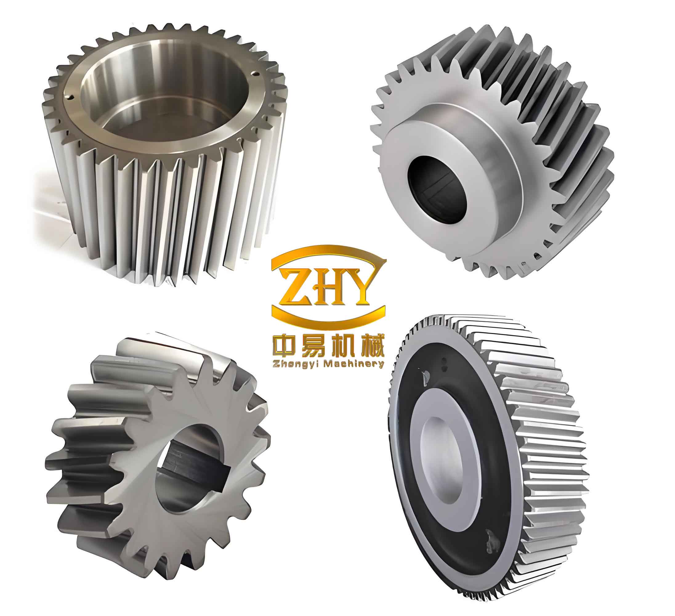
Helical gears differ from spur gears because their teeth are inclined relative to the axis. This inclination introduces an axial component of the mesh force and makes the contact line oblique in the mesh plane. The contact line length of helical gears varies continuously during a meshing cycle. Therefore, the mesh stiffness of helical gears cannot be obtained by simply extending the spur gear formulas. I observed that many existing analytical models for helical gears overly simplify the tooth profile, ignore the dependency of Hertzian contact stiffness on the contact force, repeatedly count the foundation stiffness when multiple tooth pairs mesh simultaneously, or neglect the effect of the axial force. These simplifications reduce the accuracy of the time-varying mesh stiffness of helical gears and limit the reliability of subsequent dynamic analysis.
I also noticed that pitting and spalling faults are usually modeled as rectangular or circular depressions with constant depth. Such models are convenient but are not consistent with real pitting shapes. Real pitting in helical gears often has an ellipsoidal, curved-bottom, or irregular surface. The fault shape directly affects the effective contact line, the cross-sectional area, the area moment of inertia, and the Hertzian contact condition. Therefore, I propose three pitting models: a special ellipsoid model, a general ellipsoid model, and an irregular pitting model. These models allow me to evaluate the time-varying mesh stiffness of helical gears under more realistic fault conditions.
In addition, I investigate the compound transmission stiffness of a shaft-gear assembly. In many dynamic models, the shaft and the gear pair are treated separately. However, the shaft and the gear pair are connected in a coupled manner. Because the pinion and gear have different numbers of teeth, the torque and rotational angle on the two sides are related by the transmission ratio. I therefore derive a compound transmission stiffness formula based on the total twist angle. I also design an experimental platform to measure the twist angle and to validate the proposed formula.
Finally, I build a thirteen-degree-of-freedom dynamic model of a helical gear transmission system. This model includes the rotational degrees of freedom of the motor, pinion, gear, and load, as well as the translational degrees of freedom of the pinion, gear, and gearbox in three directions. I include the friction excitation caused by mixed elastohydrodynamic lubrication and the coupling effect of the gearbox. I solve the dynamic equations using a stiff solver and analyze the time-domain and frequency-domain responses of the system under healthy and pitting conditions. The results show that pitting in helical gears produces periodic changes in the dynamic mesh force, friction force, friction moment, and gearbox acceleration. Sidebands appear around the mesh frequency, and their amplitude and distribution are related to the pitting severity.
2. Analytical Time-Varying Mesh Stiffness of Healthy Helical Gears
I calculate the time-varying mesh stiffness of helical gears by combining the slicing principle with the potential energy method. I divide the helical gear into many thin slices along the tooth width. Because each slice is very thin, the helix angle effect within one slice is negligible, and the slice can be treated as a spur gear slice. The total mesh stiffness of helical gears is then obtained by summing the contributions of all engaged slices. This approach allows me to capture the variation of the contact line length and the change in the number of engaged slices.
The end-face parameters of helical gears are related to the normal parameters by the helix angle. I use the following relations:
$$
m_t = \frac{m_n}{\cos\beta}
$$
$$
p_t = \frac{p_n}{\cos\beta}
$$
$$
\tan\alpha_t = \frac{\tan\alpha_n}{\cos\beta}
$$
$$
\tan\beta_b = \tan\beta \cos\alpha_t
$$
Here, \(m_n\) is the normal module, \(m_t\) is the transverse module, \(\beta\) is the helix angle, \(\beta_b\) is the base helix angle, \(\alpha_n\) is the normal pressure angle, and \(\alpha_t\) is the transverse pressure angle. These definitions are essential for the tooth profile equation and for the mesh stiffness of helical gears.
The tooth profile of a single slice consists of a transition curve and an involute curve. The transition curve is generated by the rounded corner of the rack cutter, while the involute curve is generated by the straight edge of the cutter. I use the following equation for the transition curve:
$$
\begin{array}{l}
x = r – r_{tr} \cos\phi + A \sin\phi \\
y = r – r_{tr} \sin\phi + A \cos\phi
\end{array}
$$
where \(r\) is the pitch radius, \(r_{tr}\) is the cutter tip radius, \(A\) is a geometric parameter of the cutter, and \(\phi\) is the parameter of the transition curve. For the involute curve, I use the standard involute equation. For any point \(K\) on the involute, the coordinates are
$$
\begin{array}{l}
x_K = r_K \cos\left(\frac{\pi}{2} – \theta_K – N_K\right) \\
y_K = r_K \sin\left(\frac{\pi}{2} – \theta_K – N_K\right)
\end{array}
$$
where \(r_K\) is the radius at point \(K\), \(\theta_K\) is the involute angle, and \(N_K\) is an orientation angle. The radius \(r_K\) is related to the base radius \(r_b\) by
$$
r_K = \frac{r_b}{\cos\alpha_K}
$$
and the involute angle is
$$
\theta_K = \tan\alpha_K – \alpha_K
$$
These equations allow me to construct the exact tooth profile of a single slice of helical gears. I then discretize the tooth profile and calculate the geometric parameters needed for the potential energy method.
The contact line of helical gears is not parallel to the gear axis. During meshing, the contact line enters from one end face and leaves from the other end face. Therefore, the length of the contact line changes with the rotation angle. The total contact ratio of helical gears is the sum of the transverse contact ratio and the overlap contact ratio:
$$
\epsilon_\gamma = \epsilon_\alpha + \epsilon_\beta
$$
The transverse contact ratio is
$$
\epsilon_\alpha = \frac{1}{2\pi}\left[N_1(\tan\alpha_{at1} – \tan\alpha_t) + N_2(\tan\alpha_{at2} – \tan\alpha_t)\right]
$$
and the overlap contact ratio is
$$
\epsilon_\beta = \frac{W \sin\beta}{\pi m_n}
$$
where \(W\) is the tooth width, \(N_1\) and \(N_2\) are the numbers of teeth of the pinion and gear, and \(\alpha_{at1}\) and \(\alpha_{at2}\) are the tip pressure angles. For helical gears with \(\epsilon_\gamma > 2\), more than two tooth pairs can mesh simultaneously. In my model, I consider the cases \(\epsilon_\beta \le \epsilon_\alpha\) and \(\epsilon_\beta \ge \epsilon_\alpha\). Depending on the contact ratio, the single tooth pair contact line length can be written in a piecewise form. For example, when \(\epsilon_\beta \le \epsilon_\alpha\), I use
$$
L(t)=
\begin{array}{l}
t/\sin\beta_b \quad \text{for } t_1 \le t \le t_2 \\
W/\cos\beta_b \quad \text{for } t_2 \le t \le t_5 \\
((t_6-t)2\pi/N_1)/\sin\beta_b \quad \text{for } t_5 \le t \le t_6
\end{array}
$$
where \(t_1, t_2, t_5, t_6\) are transition times determined by the contact ratio and the tooth width. When \(\epsilon_\beta \ge \epsilon_\alpha\), a similar piecewise expression is used with the transverse contact ratio controlling the middle interval. The total contact line at any instant is the sum of the contact lines of all engaged tooth pairs:
$$
L_{\text{total}}(t)=\sum_{i=1}^{5} L_i(t)
$$
The potential energy method divides the total elastic energy into several parts. For a single tooth pair, the total potential energy is
$$
U_{\text{total}} = U_{fp} + U_{tp} + U_h + U_{fg} + U_{tg}
$$
where \(U_{fp}\) and \(U_{fg}\) are the foundation energies of the pinion and gear, \(U_{tp}\) and \(U_{tg}\) are the tooth energies, and \(U_h\) is the Hertzian contact energy. The tooth energy itself contains the axial compression energy, bending energy, and shear energy:
$$
U_{tp} = U_{ap} + U_{bp} + U_{sp}
$$
Using Timoshenko beam theory, I express the axial compression stiffness, bending stiffness, and shear stiffness as
$$
k_a = \left(\int \frac{\sin^2\alpha}{EA_x} dx\right)^{-1}
$$
$$
k_b = \left(\int \frac{(x-x_K)^2}{EI_y} dx\right)^{-1}
$$
$$
k_s = \left(\int \frac{1.2\cos^2\alpha}{GA_x} dx\right)^{-1}
$$
where \(E\) is Young’s modulus, \(G\) is the shear modulus, \(A_x\) is the cross-sectional area, and \(I_y\) is the area moment of inertia. For a slice of thickness \(dw\), the cross-sectional area and inertia are
$$
A_x = 2y dw
$$
$$
I_y = \frac{1}{12}(2y)^3 dw
$$
The tooth stiffness of a single slice is obtained by combining these components:
$$
k_t = \left(\frac{1}{k_a} + \frac{1}{k_b} + \frac{1}{k_s}\right)^{-1}
$$
For the Hertzian contact stiffness, I use a nonlinear expression that depends on the contact force. This is important because the load sharing among multiple tooth pairs in helical gears is not uniform. I use
$$
k_h = 1.275 E^{0.9} w^{0.8} F_i^{0.1}
$$
where \(w\) is the slice width and \(F_i\) is the load carried by the \(i\)-th tooth pair. This formula captures the influence of the contact force on the Hertzian contact stiffness of helical gears.
The foundation stiffness is calculated using a well-known analytical formula. For a single tooth, the foundation stiffness is
$$
k_f = \frac{E W}{2\cos^2\alpha}
\left[
L^* \left(\frac{u_f}{S_f}\right)^2 + M^* \left(\frac{u_f}{S_f}\right) + P^* \left(\frac{u_f}{S_f}\right) + Q^*
\right]^{-1}
$$
where \(L^*, M^*, P^*, Q^*\) are polynomial coefficients. When multiple tooth pairs mesh simultaneously, the foundation stiffness can be overestimated if it is counted independently for each tooth pair. I therefore introduce a correction factor:
$$
k_f’ = C_f^* k_f
$$
The correction factor \(C_f^*\) is obtained from finite element results. In my model, I apply this correction to the foundation stiffness of helical gears under multi-tooth meshing conditions. The single slice stiffness is then
$$
k = \left(
\frac{1}{k_{tp}} + \frac{1}{k_{fp}} + \frac{1}{k_h} + \frac{1}{k_{tg}} + \frac{1}{k_{fg}’}
\right)^{-1}
$$
The single tooth pair stiffness is the sum of all engaged slices:
$$
K’ = \sum_{i=i_1}^{i_2} k_i
$$
Because the axial force also causes deformation in helical gears, I introduce a correction factor. The corrected single tooth pair stiffness is
$$
K = K’ \cos^2\beta_b
$$
The total time-varying mesh stiffness of helical gears is the sum of the stiffness of all meshing tooth pairs:
$$
K_n(t) = \sum_{i=1}^{5} K_i(t)
$$
This formulation provides a complete analytical method for the time-varying mesh stiffness of healthy helical gears.
3. Parameter Study of Healthy Helical Gears
I study how the geometric parameters of helical gears affect the mesh stiffness. The parameters include the normal module, helix angle, tooth width, pressure angle, and inner hole radius. The baseline parameters are listed in the following table.
| Parameter | Symbol | Value |
|---|---|---|
| Number of teeth | N1, N2 | 34, 52 |
| Normal module | mn | 2 mm |
| Tooth width | W | 12 mm |
| Normal pressure angle | αn | 20° |
| Helix angle | β | 15° |
| Addendum coefficient | ha* | 1 |
| Clearance coefficient | c* | 0.25 |
| Young’s modulus | E | 2.0×10^11 Pa |
| Poisson’s ratio | ν | 0.3 |
| Inner radius | ri | 15 mm |
| Applied torque | T | 100 N·m |
| Total contact ratio | εγ | 2.1321 |
When the normal module increases, the overlap contact ratio decreases, while the transverse contact ratio remains nearly constant. As a result, the meshing period of a single tooth pair becomes shorter. I find that the single tooth pair mesh stiffness decreases with increasing module. This occurs because the gear radii increase, and the circumferential force, normal force, and axial force decrease for a fixed torque. The Hertzian contact stiffness also decreases. Although the foundation stiffness increases, the overall trend is a reduction in mesh stiffness.
When the helix angle increases, the transverse contact ratio decreases, but the overlap contact ratio increases. The total contact ratio therefore increases. The normal mesh force and axial force increase because they are inversely proportional to the cosine of the helix angle. The deformation of the tooth increases, and the single tooth pair stiffness decreases. However, the total mesh stiffness of helical gears does not change dramatically because the contact ratio increases at the same time.
When the tooth width increases, the overlap contact ratio increases significantly. The single tooth pair stiffness and the total mesh stiffness both increase. This is because the load per unit width decreases, and the deformation of the tooth becomes smaller. The number of engaged slices also increases, which further raises the total stiffness of the helical gears.
When the pressure angle increases, the transverse contact ratio decreases, and the total contact ratio decreases. The tooth stiffness components, especially the bending and shear stiffness, increase with pressure angle. Therefore, both the single tooth pair stiffness and the total mesh stiffness increase. I summarize these trends in the following table.
| Parameter | Change | Effect on single tooth stiffness | Effect on total stiffness |
|---|---|---|---|
| Module | Increase | Decrease | Decrease |
| Helix angle | Increase | Slight decrease | Small variation |
| Tooth width | Increase | Increase | Increase |
| Pressure angle | Increase | Increase | Increase |
| Inner radius | Increase | Increase | Increase |
I also examine the effect of the inner hole radius. The foundation stiffness formula is valid within a certain range of the ratio between the root radius and the inner radius. For the helical gears studied here, the root radius is about 32.70 mm. I select inner radii of 10 mm, 13 mm, and 16 mm. As the inner radius increases, the foundation deformation decreases, and the foundation stiffness increases. Therefore, both the single tooth pair stiffness and the total mesh stiffness of helical gears increase. This effect is important for lightweight gear design, where hollow shafts and thin-walled gears are common.
4. Finite Element Validation of Healthy Helical Gears
I validate the proposed analytical method using finite element analysis. I build a three-dimensional model of a helical gear pair. The model includes five tooth pairs to ensure that all possible simultaneous meshing conditions are captured. I assign the material properties according to the table above. I define the contact surfaces as frictional contact with a friction coefficient of 0.2. I use a multi-zone method to generate hexahedral meshes and refine the mesh near the contact surfaces. I fix the gear completely and allow the pinion to rotate only about its axis. I apply a torque of 100 N·m to the pinion. I use a remote point on the inner surface of the pinion to obtain the loaded rotation angle. The finite element mesh stiffness is then calculated as
$$
k_{\text{finite}} = \frac{T}{r_b \theta_p}
$$
The comparison between the analytical method and the finite element method is shown in the following table. The maximum error is 1.71%. This confirms that the proposed analytical method can accurately calculate the time-varying mesh stiffness of healthy helical gears.
| Method | Maximum stiffness | Minimum stiffness | Error |
|---|---|---|---|
| Proposed analytical method | 1.75×10^8 N/m | 1.52×10^8 N/m | 1.71% |
| Finite element method | 1.78×10^8 N/m | 1.54×10^8 N/m | Reference |
5. Time-Varying Mesh Stiffness of Helical Gears with Pitting
Pitting and spalling reduce the effective contact line length of helical gears. They also alter the cross-sectional area and the area moment of inertia in the fault region. I propose an equivalent area method to account for these changes. The key idea is to replace the actual pitting cross-section with an equivalent rectangular reduction. The equivalent height \(h_s\) is obtained by dividing the reduced area by the local pitting length. This equivalent height is then used to calculate the reduced cross-sectional area and inertia of each slice.
I develop three pitting models. The first model is a special ellipsoid model. In this model, the ellipse formed by the intersection of the ellipsoid and the tooth surface is parallel to the mesh line. The ellipsoid equation is
$$
\frac{x’^2}{a^2} + \frac{y’^2}{b^2} + \frac{z’^2}{c^2} = 1
$$
For the special ellipsoid model, I set \(a = b\). The reduced area at a given mesh position is obtained by integrating the ellipse equation. The equivalent height is
$$
h_s = \frac{A_{xsk}}{l_{xsk}}
$$
where \(A_{xsk}\) is the reduced area and \(l_{xsk}\) is the local pitting length. The cross-sectional area and inertia of a slice in the pitting region are
$$
A_{xs} = (2y_s – h_s) dw
$$
$$
I_{xs} = \frac{1}{12} dw (2y_s – h_s)^3
$$
The tooth stiffness components in the pitting region are then calculated using these reduced properties. For example, the bending stiffness becomes
$$
k_{bs} = \left(
\int \frac{(x-x_K)^2}{E I_{xs}} dx
\right)^{-1}
$$
The axial compression stiffness and shear stiffness are modified in a similar way. The tooth stiffness of a slice in the pitting region is
$$
k_{ts} = \left(\frac{1}{k_{as}} + \frac{1}{k_{bs}} + \frac{1}{k_{ss}}\right)^{-1}
$$
The single slice stiffness in the pitting region is
$$
k_{\text{total},s} = \left(
\frac{1}{k_{ts}} + \frac{1}{k_{fp}} + \frac{1}{k_{tg}} + \frac{1}{k_{fg}’}
\right)^{-1}
$$
The single tooth pair stiffness in the pitting region is the sum of the healthy slices and the pitting slices. The total stiffness of helical gears with pitting is then obtained by summing the stiffness of all engaged tooth pairs. The corrected single tooth pair stiffness is
$$
K_s = K’_s \cos^2\beta_b
$$
where \(K’_s\) is the sum of the slice stiffnesses, including the reduced stiffness in the pitting region.
The second model is a general ellipsoid model. In this model, the ellipse formed by the intersection of the ellipsoid and the tooth surface is not parallel to the mesh line. The ellipse is rotated by an angle \(\alpha\). The ellipse equation in the tooth surface coordinate system is
$$
\frac{((x-x_0)\cos\alpha + (z-z_0)\sin\alpha)^2}{a^2}
+
\frac{((x-x_0)\sin\alpha – (z-z_0)\cos\alpha)^2}{c^2}
= 1
$$
I determine the pitting region by intersecting this ellipse with the mesh line. The intersection points give the local pitting length and the local pitting depth. The equivalent height is then calculated by the same area equivalence method.
The third model is an irregular pitting model. In this model, the pitting boundary is not a regular ellipse. I divide the irregular boundary into two curves along the direction perpendicular to the mesh line. I measure discrete pitting lengths and fit them with polynomial functions. The upper and lower curves are
$$
a(x) = p_n x^n + p_{n-1} x^{n-1} + \cdots + p_0
$$
$$
b(x) = q_n x^n + q_{n-1} x^{n-1} + \cdots + q_0
$$
The intersection of the mesh line with these curves gives the local pitting length. I assume a constant pitting depth for this model. The reduced area and equivalent height are then calculated in the same way as for the ellipsoid models.
I summarize the three pitting models in the following table.
| Model | Surface shape | Depth profile | Key parameter |
|---|---|---|---|
| Special ellipsoid | Ellipse parallel to mesh line | Curved bottom | a = b |
| General ellipsoid | Ellipse rotated by α | Curved bottom | Rotation angle α |
| Irregular pitting | Polynomial boundary | Constant depth | Fitted curves a(x), b(x) |
I validate the pitting models using finite element analysis. I build four models: two special ellipsoid models with different lengths, one general ellipsoid model, and one irregular pitting model. The comparison between the analytical method and the finite element method is shown in the following table. The maximum errors are 3.01%, 3.97%, 4.48%, and 2.80%, respectively. These results confirm that the proposed method can accurately calculate the time-varying mesh stiffness of helical gears with different pitting shapes.
| Pitting model | Pitting start angle | Pitting end angle | Maximum error |
|---|---|---|---|
| Special ellipsoid 1 | 7.2733° | 14.8772° | 3.01% |
| Special ellipsoid 2 | 7.2733° | 14.8772° | 3.97% |
| General ellipsoid | 7.0125° | 15.3533° | 4.48% |
| Irregular pitting | 7.0125° | 20.9535° | 2.80% |
I also compare the minimum mesh stiffness under different pitting lengths. For the first special ellipsoid model, the minimum stiffness is \(1.504 \times 10^8\) N/m. For the second special ellipsoid model, the minimum stiffness is \(1.299 \times 10^8\) N/m. The difference is 15.8%. This shows that the pitting length has a strong influence on the mesh stiffness of helical gears. As the pitting length increases, the effective contact line decreases, and the load per unit width increases. The local deformation becomes larger, and the mesh stiffness decreases further.
6. Compound Transmission Stiffness of Shaft-Gear Assemblies
In a real transmission system, the gear pair is connected to input and output shafts. The torsional stiffness of the shafts and the mesh stiffness of the gear pair together determine the transmission stiffness. I propose a compound transmission stiffness model for shaft-gear assemblies. The model treats the pinion shaft, the gear pair, and the gear shaft as a coupled system. Because the pinion and gear have different numbers of teeth, the total twist angle must account for the transmission ratio.
The total twist angle of the shaft-gear assembly is
$$
\theta_{\text{total}} = \theta_1 + \theta_{pg} + i \theta_2
$$
where \(\theta_1\) is the twist angle of the pinion shaft, \(\theta_{pg}\) is the relative twist angle of the gear pair, \(\theta_2\) is the twist angle of the gear shaft, and \(i\) is the transmission ratio. The torques are related by
$$
T_2 = i T_1
$$
Using the torsion formulas for the shafts and the mesh stiffness of the gear pair, I obtain
$$
\theta_1 = \frac{T_1}{k_1}
$$
$$
\theta_{pg} = \frac{T_1}{k_n}
$$
$$
\theta_2 = \frac{T_2}{k_2} = \frac{i T_1}{k_2}
$$
Therefore, the total twist angle is
$$
\theta_{\text{total}} = T_1 \left(\frac{1}{k_1} + \frac{1}{k_n} + \frac{i^2}{k_2}\right)
$$
The compound transmission stiffness is
$$
\frac{1}{k_{\text{total}}} = \frac{1}{k_1} + \frac{1}{k_n} + \frac{i^2}{k_2}
$$
where \(k_1\) is the torsional stiffness of the pinion shaft, \(k_2\) is the torsional stiffness of the gear shaft, and \(k_n\) is the torsional mesh stiffness of the gear pair. The torsional mesh stiffness is related to the linear mesh stiffness by
$$
k_{\text{torsional}} = r_b^2 k_{\text{rectilinear}}
$$
This relation allows me to combine the analytical mesh stiffness of helical gears with the shaft stiffness. I also consider the case of a solid gear pair. For a solid gear pair, the compound stiffness can be written as
$$
k_n = k_{\text{shaft},p} + k_{pg} + k_{\text{shaft},g}
$$
where \(k_{\text{shaft},p}\) and \(k_{\text{shaft},g}\) are the shaft stiffness contributions and \(k_{pg}\) is the gear pair stiffness. This expression is used when the gear pair is treated as a single equivalent member.
7. Experimental Platform for Compound Transmission Stiffness
I design an experimental platform to measure the compound transmission stiffness of a shaft-gear assembly. The platform consists of a support platform, a loading unit, a single-stage gearbox, a rotation angle measurement unit, and a fixed end unit. The support platform provides a stable base and has slots for fixing the loading unit. The loading unit applies a controlled torque to the pinion shaft through a lever and a force sensor. The gearbox is a commercial single-stage reducer. The fixed end unit holds the gear shaft fixed. The rotation angle measurement unit uses laser position sensors to measure the twist angles of the pinion shaft and gear shaft.
The measurement principle is based on angular amplification. The laser sensor is mounted on the shaft, and the laser spot is projected onto a wall at a known distance. When the shaft twists, the spot moves. The twist angle is calculated from the spot displacement and the distance. The total twist angle of the shaft-gear assembly is
$$
\theta_{\text{total}} = (\theta_{s1} – \theta_{s2}) + i (\theta_{s3} – \theta_{s4})
$$
where \(\theta_{s1}\) and \(\theta_{s2}\) are the measured angles on the pinion shaft, and \(\theta_{s3}\) and \(\theta_{s4}\) are the measured angles on the gear shaft. The compound transmission stiffness is then
$$
k_{\text{total}} = \frac{T}{\theta_{\text{total}}}
$$
I manufacture two shaft-gear assemblies with different gear parameters. The shaft dimensions and gear parameters are listed in the following tables.
| Shaft parameter | Symbol | Value |
|---|---|---|
| Pinion shaft length | L1 | 70 mm |
| Pinion shaft diameter | D1 | 50 mm |
| Gear shaft length | L2 | 85 mm |
| Gear shaft diameter | D2 | 60 mm |
| Gear pair | Pinion teeth | Gear teeth | Module | Tooth width |
|---|---|---|---|---|
| Pair 1 | 40 | 60 | 2.5 mm | 45 mm |
| Pair 2 | 20 | 30 | 5 mm | 45 mm |
The experimental results agree well with the theoretical predictions. The measured twist angles and the calculated compound transmission stiffness show the same trend as the analytical model. The differences are mainly caused by the compliance of the bearings, the shear and bending deformation of the shafts, and the manual loading process. I summarize the comparison in the following table.
| Gear pair | Theoretical stiffness | Experimental stiffness | Difference |
|---|---|---|---|
| Pair 1 | 1.76×10^6 N·m/rad | 1.71×10^6 N·m/rad | 2.8% |
| Pair 2 | 8.92×10^5 N·m/rad | 8.63×10^5 N·m/rad | 3.3% |
8. Thirteen-Degree-of-Freedom Dynamic Model of Helical Gears
I establish a thirteen-degree-of-freedom dynamic model for a helical gear transmission system. The model includes the rotational degrees of freedom of the motor, pinion, gear, and load, and the translational degrees of freedom of the pinion, gear, and gearbox in the x, y, and z directions. The generalized coordinate vector is
$$
\delta_M = \{ \theta_M, \theta_p, \theta_g, \theta_L, x_p, y_p, z_p, x_g, y_g, z_g, x_f, y_f, z_f \}^T
$$
The dynamic equations are derived using Newton’s second law. For the motor and pinion, the rotational equations are
$$
I_M \ddot{\theta}_M + c_{pb}(\dot{\theta}_M – \dot{\theta}_p) + k_{pb}(\theta_M – \theta_p) = T_M
$$
$$
I_p \ddot{\theta}_p + c_{pb}(\dot{\theta}_p – \dot{\theta}_M) + k_{pb}(\theta_p – \theta_M) = -R_{bp} F_{pg} – M_p
$$
For the gear and load, the rotational equations are
$$
I_g \ddot{\theta}_g + c_{gb}(\dot{\theta}_g – \dot{\theta}_L) + k_{gb}(\theta_g – \theta_L) = R_{bg} F_{pg} + M_g
$$
$$
I_L \ddot{\theta}_L + c_{gb}(\dot{\theta}_L – \dot{\theta}_g) + k_{gb}(\theta_L – \theta_g) = -T_L
$$
The translational equations for the pinion are
$$
m_p \ddot{x}_p + c_{px}(\dot{x}_p – \dot{x}_f) + k_{px}(x_p – x_f) = F_{mx} + F_{fp}
$$
$$
m_p \ddot{y}_p + c_{py}(\dot{y}_p – \dot{y}_f) + k_{py}(y_p – y_f) = F_{my} + F_{fp}
$$
$$
m_p \ddot{z}_p + c_{pz}(\dot{z}_p – \dot{z}_f) + k_{pz}(z_p – z_f) = F_{mz}
$$
The translational equations for the gear are
$$
m_g \ddot{x}_g + c_{gx}(\dot{x}_g – \dot{x}_f) + k_{gx}(x_g – x_f) = -F_{mx} – F_{fp}
$$
$$
m_g \ddot{y}_g + c_{gy}(\dot{y}_g – \dot{y}_f) + k_{gy}(y_g – y_f) = -F_{my} – F_{fp}
$$
$$
m_g \ddot{z}_g + c_{gz}(\dot{z}_g – \dot{z}_f) + k_{gz}(z_g – z_f) = -F_{mz}
$$
The equations for the gearbox are
$$
m_f \ddot{x}_f + c_{xf} \dot{x}_f + k_{xf} x_f – c_{px}(\dot{x}_p – \dot{x}_f) – k_{px}(x_p – x_f) – c_{gx}(\dot{x}_g – \dot{x}_f) – k_{gx}(x_g – x_f) = 0
$$
$$
m_f \ddot{y}_f + c_{yf} \dot{y}_f + k_{yf} y_f – c_{py}(\dot{y}_p – \dot{y}_f) – k_{py}(y_p – y_f) – c_{gy}(\dot{y}_g – \dot{y}_f) – k_{gy}(y_g – y_f) = 0
$$
$$
m_f \ddot{z}_f + c_{zf} \dot{z}_f + k_{zf} z_f – c_{pz}(\dot{z}_p – \dot{z}_f) – k_{pz}(z_p – z_f) – c_{gz}(\dot{z}_g – \dot{z}_f) – k_{gz}(z_g – z_f) = 0
$$
The dynamic mesh force is
$$
F_{pg} = k_m \delta_m + c_m \dot{\delta}_m
$$
where \(k_m\) is the total mesh stiffness of the helical gears, \(c_m\) is the mesh damping, and \(\delta_m\) is the dynamic transmission error. The mesh force components in the x, y, and z directions are
$$
F_{mx} = F_{pg} \cos\beta_b \cos\alpha
$$
$$
F_{my} = F_{pg} \cos\beta_b \sin\alpha
$$
$$
F_{mz} = F_{pg} \sin\beta_b
$$
The dynamic transmission error is related to the rotational and translational displacements by
$$
\delta_m = \frac{1}{\cos\beta_b}
\left[
R_{bp}\theta_p – R_{bg}\theta_g + (x_p – x_g)\cos\alpha + (y_p – y_g)\sin\alpha – e(t)
\right]
$$
where \(e(t)\) is the static transmission error. This model captures the coupling between the rotational and translational motions of the helical gears.
9. Friction Excitation under Mixed Elastohydrodynamic Lubrication
I include the friction excitation generated under mixed elastohydrodynamic lubrication. The friction coefficient depends on the sliding speed, rolling speed, contact pressure, oil viscosity, surface roughness, and curvature radius. I use a regression-based friction coefficient model:
$$
\mu_i = e^{b_1} S^{b_2} P_h^{b_3} V_e^{b_4} v_0^{b_5} R^{b_6} S_r^{b_7} v_r^{b_8}
$$
where \(S\) is the composite surface roughness, \(P_h\) is the Hertzian contact pressure, \(V_e\) is the entrainment velocity, \(v_0\) is the inlet oil viscosity, \(R\) is the equivalent curvature radius, \(S_r\) is the slide-to-roll ratio, and \(v_r\) is the sliding velocity. The regression coefficients are
$$
b_1 = -8.92, \quad b_2 = 1.03, \quad b_3 = 1.04, \quad b_4 = -0.35
$$
$$
b_5 = 2.81, \quad b_6 = -0.10, \quad b_7 = 0.75, \quad b_8 = -0.39
$$
The friction force on a single slice is
$$
F_{fpi} = \mu_i F_{pgi}
$$
where \(F_{pgi}\) is the normal load on the slice. The friction moments on the pinion and gear are
$$
M_{pi} = r_{pm} F_{fpi}
$$
$$
M_{gi} = r_{gm} F_{fpi}
$$
The total friction force and moments are obtained by summing over all engaged slices:
$$
F_{fp} = \sum_{i=1}^{n} F_{fpi}
$$
$$
M_p = \sum_{i=1}^{n} M_{pi}
$$
$$
M_g = \sum_{i=1}^{n} M_{gi}
$$
When pitting occurs, the surface roughness in the pitting region changes. I model this by
$$
S_{g,\text{spall}} = S_{\text{healthy}} \frac{L_{\text{spall}}}{L}
$$
where \(L_{\text{spall}}\) is the length of the pitting region and \(L\) is the total contact line length. This change in surface roughness increases the friction coefficient and the friction force. The pitting also reduces the effective contact line length, which increases the load per unit width. Both effects contribute to the dynamic response of the helical gears.
10. Dynamic Response under Healthy Conditions
I solve the dynamic equations using a stiff solver. The key parameters of the system are listed in the following tables.
| Parameter | Value |
|---|---|
| Pinion teeth | 34 |
| Gear teeth | 52 |
| Pinion mass | 0.303 kg |
| Gear mass | 0.802 kg |
| Gearbox mass | 18.509 kg |
| Pinion inertia | 2.2265×10^-4 kg·m² |
| Gear inertia | 1.252963×10^-3 kg·m² |
| Motor inertia | 0.020356 kg·m² |
| Load inertia | 0.007585 kg·m² |
| Input torque | 100 N·m |
| Output torque | 152.94 N·m |
| Pinion shaft torsional stiffness | 30585 N·m/rad |
| Gear shaft torsional stiffness | 30585 N·m/rad |
| Gearbox x stiffness | 1.9912×10^8 N/m |
| Gearbox y stiffness | 2.036×10^8 N/m |
| Gearbox z stiffness | 1.9512×10^7 N/m |
| Bearing parameter | x direction | y direction | z direction |
|---|---|---|---|
| Pinion bearing stiffness | 6.2×10^7 N/m | 6.2×10^7 N/m | 3.0×10^7 N/m |
| Gear bearing stiffness | 6.2×10^7 N/m | 6.2×10^7 N/m | 3.0×10^7 N/m |
| Pinion bearing damping | 1.5×10^4 Ns/m | 1.5×10^4 Ns/m | 7.5×10^3 Ns/m |
| Gear bearing damping | 1.5×10^4 Ns/m | 1.5×10^4 Ns/m | 7.5×10^3 Ns/m |
For a rotational speed of 6000 rpm, the theoretical mesh frequency is
$$
f_m = \frac{n N_1}{60} = \frac{6000 \times 34}{60} = 3400 \text{ Hz}
$$
The input shaft frequency is
$$
f_s = \frac{n}{60} = 100 \text{ Hz}
$$
The output shaft frequency is
$$
f_{s1} = \frac{f_s}{i} = 65.4 \text{ Hz}
$$
The dynamic mesh force under healthy conditions fluctuates around 56500 N. The theoretical value is 54647 N. The frequency spectrum of the dynamic mesh force shows a dominant peak at 340.1 Hz, which is very close to the theoretical mesh frequency. This validates the dynamic model.
The friction force and friction moment vary periodically. The curvature radius of the pinion increases during meshing, while the curvature radius of the gear decreases. The sum of the two curvature radii remains constant. The friction force changes sign as the contact point crosses the pitch line. The friction moments on the pinion and gear are different because the curvature radii are different.
The displacement, velocity, and acceleration responses of the pinion, gear, and gearbox are obtained. The pinion and gear have larger vibration amplitudes than the gearbox. The gearbox is fixed by bolts, so its vibration amplitude is small. The acceleration response of the gearbox is especially important because in practical measurements the sensors are mounted on the gearbox surface. The frequency spectrum of the gearbox acceleration shows peaks at the mesh frequency and its harmonics.
11. Dynamic Response under Pitting Conditions
I simulate four pitting conditions: two general ellipsoid models with different lengths, one special ellipsoid model, and one irregular pitting model. The dynamic mesh force, friction force, friction moment, and gearbox acceleration are analyzed.
Under pitting conditions, the dynamic mesh force exhibits periodic fluctuations. As the pitting length increases, the fluctuation amplitude increases. This is because the pitting reduces the effective contact line and the mesh stiffness of the helical gears. The load per unit width increases, and the dynamic mesh force becomes more uneven. The pitting also changes the surface roughness, which increases the friction coefficient and the friction force.
The friction force and friction moment in the pitting region are larger than in the healthy region. The friction moment on the pinion and gear increases with the pitting length. The irregular pitting model produces a more complex friction response because its boundary is not regular.
The gearbox acceleration also shows periodic impacts under pitting conditions. The impact occurs when the contact point passes through the pitting region. The amplitude of the acceleration increases with the pitting severity. In the frequency domain, sidebands appear around the mesh frequency. The sidebands are caused by the periodic impact of the pitting fault. The modulation sidebands extend over a wide frequency range, and their amplitude increases with the pitting length. This behavior is consistent with the characteristics of localized faults in helical gears.
I summarize the dynamic response characteristics under different pitting conditions in the following table.
| Pitting condition | Mesh force fluctuation | Friction force | Gearbox acceleration | Sidebands |
|---|---|---|---|---|
| General ellipsoid 1 | Moderate | Moderate increase | Moderate impact | Clear sidebands |
| General ellipsoid 2 | Large | Large increase | Large impact | Wider sidebands |
| Special ellipsoid | Moderate | Moderate increase | Moderate impact | Clear sidebands |
| Irregular pitting | Complex | Complex variation | Strong impact | Broad sidebands |
12. Discussion
The results show that the time-varying mesh stiffness of helical gears is strongly affected by the tooth geometry, the contact line variation, the load distribution, and the pitting shape. The proposed slicing method combined with the potential energy method provides a reliable way to calculate the mesh stiffness of helical gears. The nonlinear Hertzian contact stiffness and the foundation stiffness correction are essential for accurate results. The axial force correction further improves the accuracy.
The pitting models demonstrate that the fault shape has a significant influence on the mesh stiffness of helical gears. Rectangular and circular models may underestimate or overestimate the stiffness reduction. The ellipsoid and irregular models provide more realistic results. The equivalent area method is effective for handling curved-bottom and irregular pitting shapes.
The compound transmission stiffness model shows that the shaft and gear pair cannot be treated as independent components. The transmission ratio must be included in the total twist angle calculation. The experimental platform validates the proposed formula and provides a practical way to measure the compound transmission stiffness of shaft-gear assemblies.
The thirteen-degree-of-freedom dynamic model shows that the friction excitation and gearbox coupling significantly affect the vibration response of helical gears. The friction force and friction moment vary periodically and introduce additional harmonics. The gearbox acceleration is a good indicator of pitting faults because it is sensitive to the periodic impacts caused by the pitting region. The sidebands around the mesh frequency can be used for fault detection and severity assessment.
13. Conclusion
I have developed an improved analytical method for the time-varying mesh stiffness of helical gears. The method considers the nonlinear Hertzian contact stiffness, the foundation stiffness correction under multi-tooth meshing, and the axial force effect. I validated the method using finite element analysis, and the maximum error is 1.71%. I also studied the influence of module, helix angle, tooth width, pressure angle, and inner radius on the mesh stiffness of helical gears.
I proposed three pitting models for helical gears: a special ellipsoid model, a general ellipsoid model, and an irregular pitting model. I introduced an equivalent area method to calculate the reduced cross-sectional area and inertia in the pitting region. The results show that pitting reduces the mesh stiffness of helical gears, and the reduction depends on the pitting shape, length, and orientation. The maximum error between the analytical method and finite element method is less than 4.5%.
I derived a compound transmission stiffness formula for shaft-gear assemblies. The formula accounts for the transmission ratio and the torsional stiffness of the shafts and the gear pair. I designed an experimental platform and manufactured two shaft-gear assemblies to validate the formula. The experimental results agree well with the theoretical predictions.
I established a thirteen-degree-of-freedom dynamic model for helical gears. The model includes the rotational and translational degrees of freedom of the system, the friction excitation under mixed elastohydrodynamic lubrication, and the gearbox coupling. The dynamic mesh force, friction force, friction moment, and gearbox acceleration were analyzed under healthy and pitting conditions. The results show that pitting causes periodic impacts, increases the friction force and moment, and produces sidebands around the mesh frequency. These features are useful for fault diagnosis and severity assessment of helical gears.
Overall, the proposed methods provide a comprehensive framework for the mesh stiffness calculation and dynamic analysis of helical gears with pitting. The framework can be extended to other gear faults and transmission configurations in future work.