
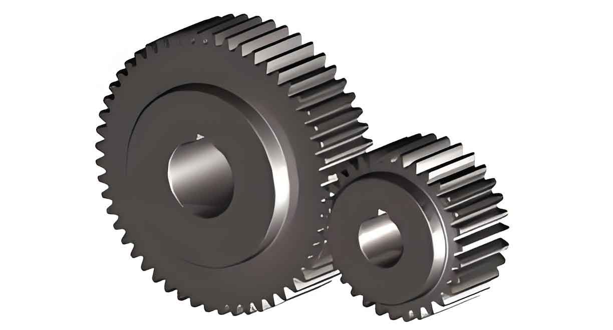
In the realm of mechanical power transmission, spur gears remain a fundamental component. Their reliability and efficiency are paramount to the overall performance of countless systems, from automotive drivetrains to industrial machinery and mining equipment like shearer ranging arms. A persistent challenge in spur gear design and operation is the dynamic excitation caused by fluctuating mesh stiffness. As gear teeth engage and disengage, the number of tooth pairs in contact alternates between one and two (for non-integer contact ratios), leading to periodic variations in the overall stiffness of the gear mesh. This stiffness variation acts as a primary internal excitation source, inducing vibration and noise, which can ultimately compromise system reliability and lifespan.
One highly effective method to mitigate this problem is tooth profile modification. The principle involves intentionally and slightly altering the ideal involute profile, typically by removing a small amount of material from the tip and/or root regions of the gear tooth. This strategic removal aims to compensate for elastic deformations, manufacturing errors, and thermal expansions that occur under load, thereby smoothing the transition of load between mating tooth pairs and reducing transmission error. In this analysis, I will delve into the intricate relationship between tooth profile modification parameters and the design transmission error of spur gears, building a comprehensive model, outlining an optimization strategy, and discussing the practical implications of various modification schemes.
Understanding Design Transmission Error in Spur Gears
Transmission Error (TE) is defined as the deviation of the actual angular position of the driven gear from its theoretical position relative to the driver gear. When we consider only the component caused by the elastic deformation of the teeth under load, excluding manufacturing and assembly errors, we refer to it as Design Transmission Error. This parameter is a direct indicator of the stiffness excitation within the gear mesh. A lower and smoother design TE waveform generally correlates with reduced dynamic forces and quieter operation.
To model this, we begin by treating each spur gear tooth as a non-uniform cantilever beam fixed at the root and loaded at the contact point. The total elastic deformation at any meshing point is a superposition of three components: bending and shear deflection of the cantilever, additional deflection due to the flexibility of the gear body (foundation), and Hertzian contact deformation at the point of contact between the two teeth.
The bending and shear deflection for a tooth loaded at point j with force \(F_j\) can be calculated by discretizing the tooth into n segments. For a segment i with thickness \(T_i\), area \(A_i\), area moment of inertia \(I_i\), and distance \(L_{ij}\) from the segment to the load point, the contribution is given by a detailed integral formulation. The foundation deflection \(\delta_{Mj}\) accounts for the non-rigid support, and the contact deflection \(\delta_{Cj}\) follows from Hertzian contact theory. The total deflection for a single tooth pair is thus:
$$\delta_j = \delta_{Bj} + \delta_{Mj} + \delta_{Cj}$$
The mesh stiffness \(k\) for a single tooth pair is the reciprocal of the sum of the deflections of the driving and driven teeth:
$$k_s = \frac{1}{\delta_z + \delta_c} = \frac{1}{\frac{1}{k_z} + \frac{1}{k_c}}$$
where \(k_z\) and \(k_c\) are the individual tooth stiffnesses of the driver and driven spur gears, respectively. The overall mesh stiffness \(k_m(\tau)\) varies with the roll angle \(\tau\) (or time) as the contact moves along the path of action. For a spur gear pair with a contact ratio \(\varepsilon\) between 1 and 2, the mesh stiffness is a periodic function switching between one and two pairs in contact:
$$
k_m(\tau) =
\begin{cases}
k_{s1}(\tau), & \tau_1 \le \tau \le \tau_2 \\
k_{s1}(\tau) + k_{s2}(\tau), & \tau < \tau_1, \tau > \tau_2
\end{cases}
$$
Here, \(\tau_1\) and \(\tau_2\) are the roll angles marking the transition points between single and double tooth contact zones, corresponding to the lowest point of single tooth contact (LPSTC) and the highest point of single tooth contact (HPSTC). Finally, the design transmission error \(\nu(\tau)\) is the ratio of the total applied load per unit face width \(w\) to the time-varying mesh stiffness:
$$
\nu(\tau) = \frac{w}{k_m(\tau)}
$$
Modeling the Impact of Tooth Profile Modification
Tooth profile modification for spur gears is defined by three key parameters: the modification amount (\(\Delta_{max}\)), the modification length (\(L\)), and the modification curve (defined by an exponent \(e\)). The modification is typically applied from a start point \(g\) on the tooth flank towards the tip (tip relief) or root (root relief).
The ideal maximum modification amount should compensate for the total expected displacement under load:
$$\Delta_{max} = \delta_j + \delta_m + \delta_t$$
where \(\delta_j\) is the load-induced elastic deformation, \(\delta_m\) accounts for manufacturing errors, and \(\delta_t\) is the thermal deformation. The modification length \(L\) is the distance along the tooth profile from the start point to the tip (or root). The amount of material removed \(\Delta(s)\) at a distance \(s\) from the start point is governed by:
$$\Delta(s) = \Delta_{max} \left( \frac{s}{L} \right)^e$$
Here, \(e=1\) represents a linear modification, while \(e=2\) represents a parabolic modification. The introduction of this modification alters the local tooth geometry. When a tooth with a modified profile enters contact, the initial contact point shifts, effectively changing the load application angle \(\beta\) to \(\beta’ = \beta – \Delta\beta\) and the local tooth thickness. This, in turn, modifies the tooth compliance calculations (\(\delta_{Bj}’, \delta_{Mj}’\)). Consequently, the single-pair stiffness \(k_s’\) and the transition points \(\tau_1′, \tau_2’\) are recalculated. The design transmission error for the modified spur gear pair then becomes:
$$
\nu'(\tau) = \frac{w}{k_m'(\tau)}
$$
$$
\text{where } k_m'(\tau) =
\begin{cases}
k_{s1}'(\tau), & \tau_1′ \le \tau \le \tau_2′ \\
k_{s1}'(\tau) + k_{s2}'(\tau), & \tau < \tau_1′, \tau > \tau_2′
\end{cases}
$$
Optimizing Spur Gear Tooth Profile Modification
To systematically improve spur gear performance, we can frame the selection of modification parameters as a multi-objective optimization problem. The primary goals are to minimize both the peak value and the fluctuation amplitude of the design transmission error, thereby reducing dynamic excitation.
Objective Functions:
1. Minimize peak transmission error: \(f_1 = \max(\nu'(\tau))\)
2. Minimize transmission error fluctuation: \(f_2 = \max(\nu'(\tau)) – \min(\nu'(\tau))\)
Design Variables:
– \(x_1 = \Delta_{max}\): Maximum modification amount (µm).
– \(x_2 = L\): Modification length (mm), which implicitly defines the start point.
– \(x_3 = e\): Modification curve exponent (1 or 2).
Constraints:
– \(\Delta_{max} \leq B/2\) (not exceeding half the tooth thickness \(B\)).
– \(L \leq h_f\) (not exceeding the dedendum \(h_f\)).
– \(e \in \{1, 2\}\).
This kind of problem, with conflicting objectives (reducing peak vs. reducing fluctuation), is well-suited for a multi-objective genetic algorithm like NSGA-II (Non-dominated Sorting Genetic Algorithm II). NSGA-II works with a population of potential solutions, uses a fast non-dominated sorting procedure to rank them based on Pareto optimality, and employs crowding distance to maintain diversity, efficiently searching for a set of optimal compromises (the Pareto front).
Case Study: Analysis of a Shearer Ranging Arm Spur Gear Drive
Let’s apply this methodology to a real-world example: the spur gear transmission system in a coal shearer ranging arm. The key parameters for the driver and driven spur gears are summarized below:
| Parameter | Driver Spur Gear | Driven Spur Gear |
|---|---|---|
| Number of Teeth | 35 | 60 |
| Module (mm) | 4 | |
| Pressure Angle (°) | 20 | |
| Face Width (mm) | 70 | |
| Contact Ratio, \(\varepsilon\) | 1.736 | |
Using measured input torque data from field testing and the models described, we can calculate the unmodified design TE. It shows characteristic sharp discontinuities at the transition points between single and double tooth contact zones, with a significant peak-to-peak variation. We then define several modification schemes to analyze the influence of each parameter, with Scheme A being the unmodified baseline.
| Scheme | Modification Amount \(\Delta_{max}\) (µm) | Modification Start Point (mm from pinion center)* | Modification Curve (e) |
|---|---|---|---|
| A (Baseline) | 0 | – | – |
| B | 3 | 25.213 (HPSTC) | 1 (Linear) |
| C | 9 | 25.213 (HPSTC) | 1 (Linear) |
| D | 16 | 25.213 (HPSTC) | 1 (Linear) |
| E | 21 | 25.213 (HPSTC) | 1 (Linear) |
| F | 9 | 23.941 (Pitch Point) | 1 (Linear) |
| G | 9 | 22.091 (LPSTC) | 1 (Linear) |
| H | 9 | 25.213 (HPSTC) | 2 (Parabolic) |
*HPSTC: Highest Point of Single Tooth Contact; LPSTC: Lowest Point of Single Tooth Contact.
Influence of Modification Amount: Comparing Schemes A through E reveals a clear trend. A small modification (3 µm, Scheme B) begins to smooth the TE curve. An optimal amount (9 µm, Scheme C) significantly reduces the fluctuation amplitude, creating a much smoother transition between engagement phases without increasing the peak error. However, excessive modification (16 µm and 21 µm, Schemes D & E) increases the peak TE and can reintroduce harshness, as too much material is removed, effectively reducing the contact ratio and changing the load distribution unfavorably.
Influence of Modification Start Point: Holding the amount at 9 µm and using a linear curve, we compare Schemes C, F, and G. Starting the modification at the HPSTC (Scheme C) yields the best result with the lowest peak TE. Starting earlier, at the pitch point (Scheme F) or even earlier at the LPSTC (Scheme G), increases the peak TE markedly and creates a double-peak waveform, indicating a less favorable load transfer and increased dynamic excitation.
Influence of Modification Curve: Comparing Scheme C (linear, e=1) and Scheme H (parabolic, e=2) with the same amount and start point shows that the parabolic profile offers a marginally smoother entry and exit of the tooth into mesh. The transition in the TE curve is very gradual. The linear modification, while still excellent, can have a slightly more abrupt change in slope at the very beginning of the modified region. The peak TE values for both are nearly identical.
Quantitative Improvement: The optimization process identifies Scheme C as a superior choice for these particular spur gears. The unmodified spur gears (Scheme A) had a TE fluctuation amplitude of 7.05 µm. The optimized modification (Scheme C) reduced this amplitude to 3.20 µm, representing a reduction of 54.6%. This dramatic smoothing directly correlates with a significant reduction in stiffness-based dynamic excitation.
Conclusions and Engineering Implications
This detailed exploration underscores the critical importance of precise tooth profile modification in the design of high-performance spur gear drives. The interaction between modification parameters and the resulting design transmission error is complex but can be systematically modeled and optimized.
The key takeaways for engineers designing spur gears are:
1. Modification Amount is Critical: There exists an optimal value. Insufficient modification leaves excitation sources unaddressed, while excessive modification degrades performance by raising the peak transmission error.
2. Start Point Defines the Peak: For spur gears aiming to minimize peak dynamic load, initiating the modification at or very near the Highest Point of Single Tooth Contact (HPSTC) is generally most effective. Starting the relief earlier tends to increase the peak error.
3. Curve Shape Affects Smoothness: Parabolic modification profiles can provide a marginally smoother engagement characteristic compared to linear profiles for spur gears, though both are effective when parameters are well-chosen.
4. A Systematic Approach is Valuable: Combining analytical or finite-element-based deformation models with multi-objective optimization algorithms like NSGA-II provides a powerful framework for determining the best modification parameters tailored to specific spur gear applications, leading to designs with inherently lower vibration and noise.
In conclusion, tooth profile modification is not merely a corrective step but a fundamental design tool for optimizing the dynamic behavior of spur gears. By carefully tailoring the modification amount, length, and curve, engineers can directly manipulate the design transmission error—the primary stiffness excitation—to create spur gear transmissions that are smoother, quieter, and more reliable.