
In this work, I systematically investigated the influence of tooth surface modification and loading meshing performance of hypoid gears on the NVH (Noise, Vibration, Harshness) behavior of an automobile drive axle. The research was motivated by the practical need to suppress high-speed whining in the rear axle, which is directly related to the meshing quality of the hypoid gear pair. My approach combined mathematical modeling, numerical tooth surface generation, finite element loading contact analysis, drive axle NVH simulation, and experimental validation. I proposed a pre-controlled Ease-off topology modification method, and demonstrated through both simulation and experiments that the modified tooth surface significantly improves the NVH performance of the drive axle.
Hypoid gears are widely used in automobile drive axles because of their large contact ratio, smooth transmission, and high load-carrying capacity. However, under actual working conditions, the gear pair is subjected to load-induced misalignment, which changes the contact pattern and transmission error, often leading to unacceptable noise and vibration. To address this issue, I developed a complete methodology for tooth surface design and modification, focusing on the pinion tooth surface, and then evaluated the influence of the modified surface on the drive axle NVH response.
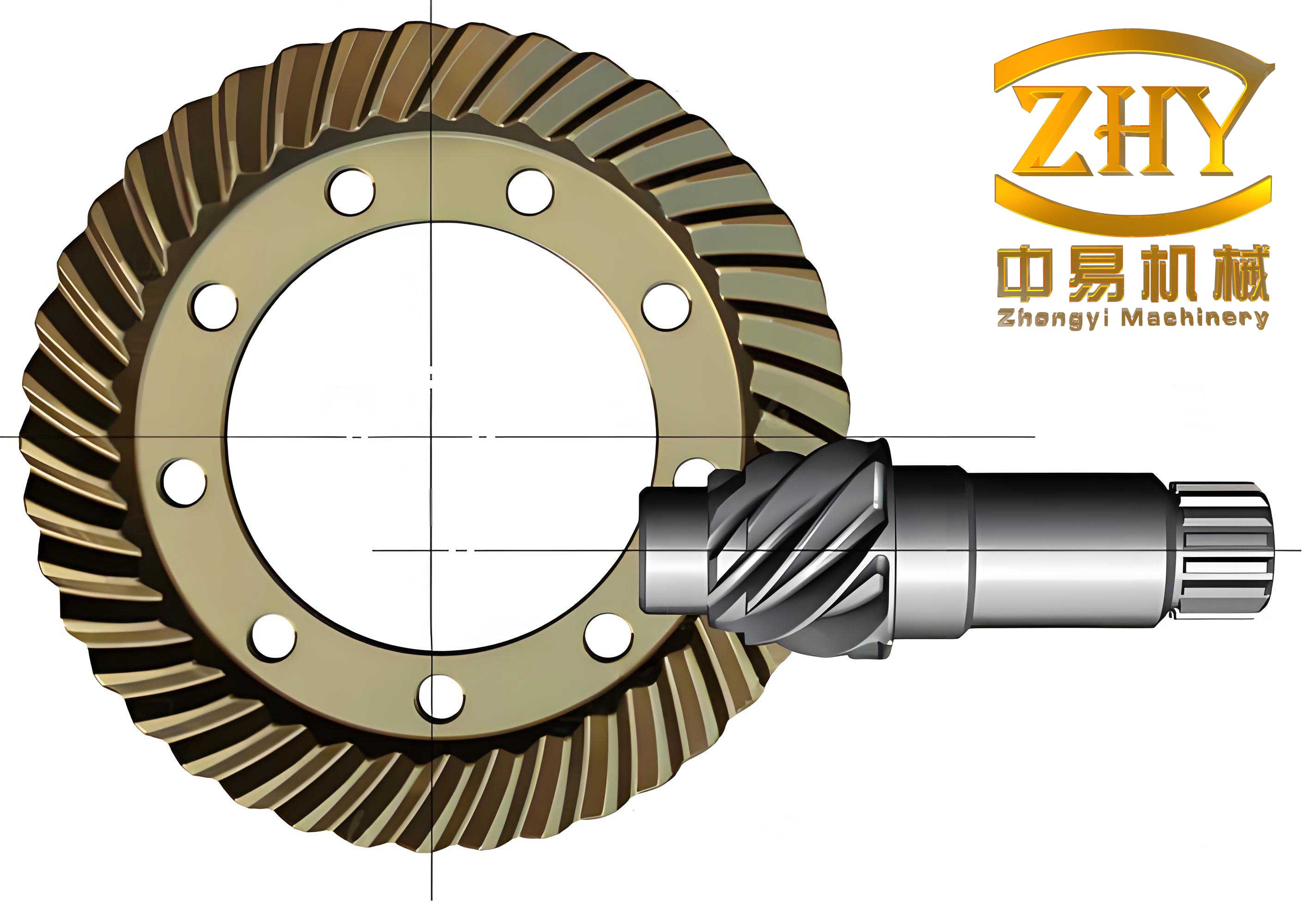
1. Numerical Tooth Surface Calculation and 3D Modeling of Hypoid Gears
I first established the machining mathematical model for hypoid gears manufactured by the HFT (Hypoid Formate Tilt) method. In this method, the gear is produced by the formate process while the pinion is generated by the tilt process. The pinion tooth surface equation was derived from the tool surface equation through a series of coordinate transformations. I defined the tool coordinate system for the pinion cutter head, as commonly used in face-milled hypoid gear production. The tool surface for the inner and outer blades can be expressed in the cutter coordinate system as:
$$
\mathbf{r}_k(u_k, \theta_k) =
\begin{bmatrix}
(r_k + u_k \sin\alpha_k)\cos\theta_k \\
(r_k + u_k \sin\alpha_k)\sin\theta_k \\
-c_k + u_k \cos\alpha_k \\
1
\end{bmatrix}
$$
where $k = g$ denotes the inner blade and $k = p$ denotes the outer blade, $r_k$ is the tip radius, $\alpha_k$ is the blade angle, $u_k$ is the blade surface parameter, and $c_k$ is a constant offset. The unit normal vector is given by:
$$
\mathbf{n}_k = \frac{\partial \mathbf{r}_k/\partial \theta_k \times \partial \mathbf{r}_k/\partial u_k}{\left| \partial \mathbf{r}_k/\partial \theta_k \times \partial \mathbf{r}_k/\partial u_k \right|}
$$
By applying the machine kinematics of the tilt method, including the tilt angle $i$, swivel angle $j$, radial setting $S_{r1}$, angular setting $q_1$, vertical offset $E_{m1}$, bed correction $X_{b1}$, axial correction $X_{p1}$, machine root angle $\gamma_1$, and the roll ratio $R_b$, I transformed the tool surface to the machine coordinate system and then to the pinion coordinate system. The meshing condition between the tool and the pinion blank is expressed as:
$$
\mathbf{n}_m \cdot \mathbf{v}_m^{(c1)} = 0
$$
where $\mathbf{v}_m^{(c1)}$ is the relative velocity between the cutter and the workpiece. Solving this equation eliminates one parameter and yields the pinion tooth surface $\mathbf{r}_1(u_1, \theta_1)$.
For the gear, I used the formate process, where the gear tooth surface is generated by a simple plunge motion of the cutter. The gear tooth surface equation was obtained by transforming the cutter surface into the gear coordinate system, leading to $\mathbf{r}_2(u_2, \theta_2)$. I also derived the transition surface equation for the tooth root fillet, which is essential for accurately predicting root bending stress. The transition surface was generated by the tool tip radius and can be written as:
$$
\mathbf{r}_g'(u_w, \beta, \theta_w) =
\begin{bmatrix}
(r_w + u_0 \sin\alpha_w + r_0(\sin\alpha_w \cos\beta – \cos\alpha_w \sin\beta))\cos\theta_w \\
(r_w + u_0 \sin\alpha_w + r_0(\sin\alpha_w \cos\beta – \cos\alpha_w \sin\beta))\sin\theta_w \\
u_0 \cos\alpha_w + r_0(\cos\alpha_w \sin\beta – \sin\alpha_w \cos\beta) \\
1
\end{bmatrix}
$$
To compute the discrete tooth surface points, I applied the spatial rotation projection method. The tooth surface was projected onto a plane perpendicular to the gear axis, and a grid of $5 \times 9$ points was defined in the height and length directions. By solving the relationships between the 3D surface points and their projected coordinates, I obtained the coordinates of all grid points. As an example, for a point $P_{35}$ on the pinion, the following equations were solved:
$$
x_P(u,\theta) = X_{35}, \quad \sqrt{y_P^2(u,\theta) + z_P^2(u,\theta)} = Y_{35}
$$
Using the geometric and machining parameters listed in the following tables, I wrote MATLAB programs to compute the tooth surface coordinates. Table 1 gives the basic geometric parameters of the hypoid gear pair used in this study.
| Parameter | Pinion | Gear |
|---|---|---|
| Number of teeth | 8 | 39 |
| Hand of spiral | Left | Right |
| Shaft angle (deg) | 90 | |
| Offset distance (mm) | 35 (lower offset) | |
| Module (mm) | 6.283 | |
| Reference spiral angle (deg) | 50.24 | 31.37 |
| Pressure angle (deg) | 22.5 | 22.5 |
| Face width (mm) | 44.4 | 38 |
| Whole depth (mm) | 12.15 | 11.89 |
| Addendum (mm) | 8.99 | 1.59 |
| Pitch angle (deg) | 13.1 | 76.2 |
| Face angle (deg) | 18.3 | 77.13 |
| Root angle (deg) | 12.2 | 70.75 |
The machining parameters are listed in Table 2. These values were used both in the numerical tooth surface generation and in the subsequent finite element models.
| Parameter | Pinion concave | Pinion convex | Gear |
|---|---|---|---|
| Cutter tip radius (mm) | 108.075 | 120.395 | 114.3 (cutter width 3.12) |
| Tip fillet radius (mm) | 1.297 | 1.297 | 1.397 |
| Blade angle (deg) | -31 | 14 | 22.5 (concave), -22.5 (convex) |
| Tilt angle (deg) | 15.57 | 12.02 | 0 |
| Swivel angle (deg) | 320.32 | 331.28 | 0 |
| Radial setting (mm) | 104.4274 | 103.64879 | 109.058 |
| Angular setting (deg) | 82.25 | 83.3 | 67.845 |
| Machine root angle (deg) | 355.96 | 359.4 | 69.79 |
| Vertical offset (mm) | 35.86444 | 26.43132 | 0 |
| Axial setting (mm) | -1.54323 | 4.04764 | 0.8075 |
| Bed setting (mm) | 23.62655 | 15.18808 | 0 |
| Roll ratio | 4.6933 | 4.666443 | 0 |
After computing the discrete tooth surface points, I imported them into UG (Unigraphics) to build the solid models of the pinion and gear. The procedure included creating the gear blank, generating the tooth surfaces from point clouds, creating the transition surfaces, and finally arraying the tooth slots to obtain the complete gear models. The assembled gear pair is shown in Figure 1 (inserted earlier).
2. Finite Element Loading Contact Analysis and NVH Simulation
2.1 Tooth Contact Analysis (TCA)
I established the meshing coordinate system for the hypoid gear pair, considering the shaft angle of 90°, the offset distance, and possible misalignments. The gear tooth surfaces are represented in the fixed coordinate system as:
$$
\mathbf{r}_a^{(1)}(u_1,\theta_1,\phi_1) = \mathbf{M}_{ad}\mathbf{M}_{d1}\mathbf{r}_1(u_1,\theta_1)
$$
$$
\mathbf{r}_a^{(2)}(u_2,\theta_2,\phi_2) = \mathbf{M}_{ab}\mathbf{M}_{b2}\mathbf{r}_2(u_2,\theta_2)
$$
At any instant, the two surfaces are tangent, so their position vectors and normals coincide:
$$
\mathbf{r}_a^{(1)} = \mathbf{r}_a^{(2)}, \quad \mathbf{n}_a^{(1)} = \mathbf{n}_a^{(2)}
$$
These vector equations provide five independent scalar equations with six unknowns. By fixing the pinion rotation angle $\phi_1$, I solved for the other five unknowns and obtained a series of contact points. The transmission error is defined as:
$$
\Delta\phi_2(\phi_1) = \phi_2 – \frac{z_1}{z_2}\phi_1 – (\phi_2^{(0)} – \frac{z_1}{z_2}\phi_1^{(0)})
$$
Using the parameters in Tables 1 and 2, I computed the TCA results for both the concave and convex sides of the gear. The contact pattern and transmission error curve were obtained, providing a baseline for the subsequent modification.
2.2 Finite Element Model in ABAQUS
To evaluate the loaded meshing performance, I built finite element models in ABAQUS. Since a full gear model is computationally expensive, I trimmed single-tooth segments and then assembled multiple teeth for the contact analysis. I divided the single tooth into hexahedral elements using auxiliary cutting planes. The material properties used were: elastic modulus 210000 MPa, Poisson’s ratio 0.3, and density \(7.85 \times 10^{-9}\) kg/mm³. The element type was C3D8R (reduced integration hexahedron). The mesh was refined on the tooth flank and coarser in the root and body regions.
The boundary conditions and loading were defined in three analysis steps. In the first step, the gear was fully fixed and the pinion was rotated by a small angle to establish contact. In the second step, the pinion was fixed and the gear was released to rotate about its axis to avoid overconstraint. In the third step, the pinion was driven by a prescribed rotation while the gear was free to rotate, subject to a resisting torque. A friction coefficient of 0.06 was used, and the contact was modeled as hard contact with finite sliding.
I applied the torque on the pinion and set the gear to rotate freely. For the unmodified gear pair, a torque of 50 N·m was first used. After the simulation, I wrote a Python script to extract the maximum contact stress on every element over the entire meshing cycle. The extracted values formed the complete loaded contact pattern on the gear tooth surface. The result showed that the contact pattern was an elongated ellipse with an internal diagonal orientation. The maximum contact stress was \(5.25 \times 10^3\) MPa on the gear concave side and \(5.78 \times 10^3\) MPa on the convex side.
I also extracted the actual rotation angles of the pinion and gear from the simulation. The loaded transmission error was then computed using the same definition as in TCA. The loaded transmission error curve exhibited a periodic variation with an amplitude that depends on the torque.
2.3 Drive Axle NVH Simulation in MASTA
I created a full drive axle model in MASTA to simulate the NVH behavior. The drive axle consists of the hypoid gear pair, differential, shafts, and housing. I first modeled the axle components in UG, then performed mesh generation and pre-processing in Hypermesh, and finally assembled the model in MASTA. The gear pair geometry and machining parameters were identical to those used in the ABAQUS model. The housing was represented by its stiffness and mass matrices obtained from finite element analysis in ABAQUS and then imported into MASTA.
In the NVH module, I selected the gear whine analysis option, which uses the loaded transmission error of the gear pair as the excitation source. A measurement point was placed on the housing above the pinion outer bearing, corresponding to the accelerometer position used in later road tests. The NVH analysis was performed for a torque of 50 N·m on the pinion input. The waterfall diagram was generated, and by order tracking I extracted the 8th-order vibration and noise curves. The Z-direction (vertical) response was found to be the highest, so I used that direction for evaluation.
3. Tooth Surface Modification Based on Ease-off Topology
3.1 Construction of the Reference Tooth Surface
I used the concept of a fully conjugate reference tooth surface. Given the gear tooth surface, I derived the pinion tooth surface that would mesh perfectly with the gear under zero load and zero misalignment. This reference pinion tooth surface was obtained by applying the conjugate meshing condition. In the fixed coordinate system, the gear surface is expressed as:
$$
\mathbf{r}_a^{(2)}(u_2,\theta_2,\phi_2) = \mathbf{M}_{ab}\mathbf{M}_{b2}\mathbf{r}_2(u_2,\theta_2)
$$
The meshing equation is:
$$
\mathbf{n}_a^{(2)} \cdot \mathbf{v}_a^{(21)} = 0
$$
where \(\mathbf{v}_a^{(21)}\) is the relative velocity between the gear and the pinion. Solving this equation gives \(\phi_2 = \phi_2(u_2,\theta_2)\). Substituting back, I obtained the gear surface in the fixed frame as a function of two parameters. Transforming this surface into the pinion coordinate system yielded the reference pinion tooth surface \(\mathbf{r}_1^{(0)}(u_2,\theta_2)\).
3.2 Ease-off Topology and Its Decomposition
The actual pinion tooth surface was generated from the machining model. After aligning the midpoints of the actual and reference surfaces, I computed the normal deviation between them. The deviation is called the Ease-off topology. For each point on the actual surface, the deviation \(\Delta\delta\) is calculated by projecting onto the reference surface normal:
$$
\begin{bmatrix}
x_1 – x_0 \\
y_1 – y_0 \\
z_1 – z_0
\end{bmatrix}
= \Delta\delta
\begin{bmatrix}
n_{x0} \\
n_{y0} \\
n_{z0}
\end{bmatrix}
$$
I approximated the Ease-off topology by a second-order polynomial surface:
$$
\Delta\delta = a_0 + a_1 X + a_2 Y + a_3 X^2 + a_4 Y^2 + a_5 XY
$$
where $X$ is along the face width direction and $Y$ is along the tooth height direction. The coefficients are:
- $a_0$: constant term (usually zero after midpoint alignment)
- $a_1$: spiral angle modification coefficient
- $a_2$: pressure angle modification coefficient
- $a_3$: lengthwise crowning coefficient
- $a_4$: profile crowning coefficient
- $a_5$: tooth surface twist coefficient
I collected the deviations at all grid points and solved the overdetermined system by least squares to obtain these coefficients. For the original pinion convex surface (the coast side that was studied), the computed coefficients were:
| Coefficient | Value |
|---|---|
| $a_1$ | \(-1.6208 \times 10^{-4}\) |
| $a_2$ | \(1.1 \times 10^{-3}\) |
| $a_3$ | \(-2.0301 \times 10^{-4}\) |
| $a_4$ | \(9.0264 \times 10^{-4}\) |
| $a_5$ | \(-7.0026 \times 10^{-4}\) |
3.3 Pre-controlled Modification of the Mismatch Coefficients
The Ease-off topology directly reflects the mismatch between the actual pinion and the gear. By adjusting the five coefficients, I could control the contact pattern and transmission error. For the coast side, the original gear pair exhibited an internal diagonal contact pattern and a relatively large transmission error amplitude. To improve NVH, I aimed to reduce the diagonal orientation, increase the contact area, and reduce the loaded transmission error amplitude. Accordingly, I selected new coefficient values:
| Coefficient | Original | Modified |
|---|---|---|
| $a_1$ | \(-1.6208 \times 10^{-4}\) | \(5.2 \times 10^{-4}\) |
| $a_2$ | \(1.1 \times 10^{-3}\) | \(-2.3 \times 10^{-4}\) |
| $a_3$ | \(-2.0301 \times 10^{-4}\) | \(6.9 \times 10^{-5}\) |
| $a_4$ | \(9.0264 \times 10^{-4}\) | \(5.6 \times 10^{-5}\) |
| $a_5$ | \(-7.0026 \times 10^{-4}\) | \(4 \times 10^{-5}\) |
Using these new coefficients, I constructed the desired Ease-off topology. Then, by applying the inverse of the deviation calculation, I obtained the modified target tooth surface. For each point on the reference surface, the modified surface coordinates are:
$$
\mathbf{r}_1^{(T)} = \mathbf{r}_1^{(0)} + \Delta\delta_{\text{new}} \mathbf{n}_1^{(0)}
$$
3.4 Inverse Determination of Pinion Machining Parameters
To realize the modified tooth surface in practice, I needed to determine a new set of pinion machining parameters. The actual tooth surface generated by the machining model depends on the machining parameters \(\boldsymbol{\xi} = [\xi_1, \xi_2, \ldots, \xi_k]^T\). The difference between the target surface and the actual surface can be expressed as:
$$
\mathbf{r}_1^{(T)} – \mathbf{r}_1(u,\theta,\boldsymbol{\xi}) = \delta\mathbf{r}
$$
Dotting both sides with the actual surface normal and ignoring higher-order terms gives:
$$
(\mathbf{r}_1^{(T)} – \mathbf{r}_1) \cdot \mathbf{n}_1 = \sum_{j=1}^{k} \left( \frac{\partial \mathbf{n}_1}{\partial \xi_j} \cdot \mathbf{r}_1 \right) \Delta \xi_j
$$
For each grid point $i$, the deviation is:
$$
h_i = \sum_{j=1}^{k} J_{ij} \Delta \xi_j
$$
where \(J_{ij} = (\partial \mathbf{r}_1 / \partial \xi_j) \cdot \mathbf{n}_1\) is the sensitivity coefficient. Collecting all points gives the linear system:
$$
\mathbf{h} = \mathbf{J} \Delta \boldsymbol{\xi}
$$
Since the number of grid points is larger than the number of machining parameters, this is an overdetermined system. I solved it using the sequential quadratic programming method, with constraints that kept the parameter changes within feasible limits. I selected ten machining parameters as variables: cutter tip radius, tilt angle, swivel angle, radial setting, angular setting, machine root angle, vertical offset, axial setting, bed setting, and roll ratio. The allowed ranges are summarized in Table 5.
| Parameter | Range of correction |
|---|---|
| Cutter tip radius (mm) | \(-20\) to \(+20\) |
| Tilt angle (deg) | \(-5\) to \(+5\) |
| Swivel angle (deg) | \(-15\) to \(+15\) |
| Radial setting (mm) | \(-10\) to \(+10\) |
| Angular setting (deg) | \(-10\) to \(+10\) |
| Machine root angle (deg) | \(-5\) to \(+5\) |
| Vertical offset (mm) | \(-10\) to \(+10\) |
| Axial setting (mm) | \(-10\) to \(+10\) |
| Bed setting (mm) | \(-10\) to \(+10\) |
| Roll ratio | \(-0.5\) to \(+0.5\) |
I computed the sensitivity matrix using a VC++ program. For the pinion convex surface, the sensitivity matrix was obtained. The resulting modified machining parameters are presented in Table 6.
| Parameter | Modified value | Correction |
|---|---|---|
| Cutter tip radius (mm) | 117.73 | +9.655 |
| Tilt angle (deg) | 15.90 | +0.33 |
| Swivel angle (deg) | 330.14 | +9.82 |
| Radial setting (mm) | 107.5162 | +3.0888 |
| Angular setting (deg) | 84.77 | +2.52 |
| Machine root angle (deg) | 355.98 | +0.02 |
| Vertical offset (mm) | 33.6815 | -2.18294 |
| Axial setting (mm) | 1.5049 | +0.03833 |
| Bed setting (mm) | 18.7449 | -4.88165 |
| Roll ratio | 4.6279 | -0.0654 |
After obtaining these modified parameters, I regenerated the actual pinion surface and compared it with the target surface. The maximum deviation was 2.359 μm, which is less than the required 10 μm (0.01 mm). This indicates that the actual surface is practically equivalent to the target surface.
I then performed TCA for the modified gear pair. The results showed that the contact pattern became more centralized, the diagonal orientation was reduced, the contact area increased, and the transmission error amplitude was reduced from 30 μrad to 14.8 μrad, meeting the desired NVH improvement.
4. Influence of Loading Meshing Performance on Drive Axle NVH
4.1 Calculation of Mesh Misalignment
Under actual driving conditions, the drive axle components deform under load, causing relative displacements between the pinion and gear. These displacements are called mesh misalignments and are characterized by four components: pinion axial displacement \(\Delta X_P\), gear axial displacement \(\Delta X_W\), offset change \(\Delta E\), and shaft angle change \(\Delta\Sigma\). I used MASTA to compute these values for the coast side under different negative torques corresponding to the deceleration phase of vehicle operation. The torques were \(-40\), \(-60\), \(-80\), and \(-100\) N·m. The computed misalignments are listed in Table 7.
| Torque (N·m) | \(\Delta X_P\) (μm) | \(\Delta X_W\) (μm) | \(\Delta E\) (μm) | \(\Delta\Sigma\) (μm) |
|---|---|---|---|---|
| -40 | -22.428 | 27.625 | 14.6873 | -0.0232 |
| -60 | -30.742 | 43.097 | 21.1243 | -0.0094 |
| -80 | -39.1367 | 58.9671 | 26.6865 | 0.01384 |
| -100 | -47.3308 | 74.3284 | 31.757 | 0.03851 |
These misalignments were applied as displacement constraints in the ABAQUS assembly to simulate the actual loaded contact condition.
4.2 Comparison of Loaded Tooth Contact Performance
I ran ABAQUS simulations for both the original and modified gear sets under the four torque levels. The extracted loaded contact patterns are shown qualitatively in the results. The following table summarizes the maximum contact stress values.
| Torque (N·m) | Original (MPa) | Modified (MPa) |
|---|---|---|
| -40 | 2124 | 1836 |
| -60 | 2568 | 2213 |
| -80 | 2954 | 2547 |
| -100 | 3301 | 2842 |
At every torque level, the modified tooth surface produced a lower maximum contact stress than the original. Additionally, the contact area was larger and the diagonal orientation was less pronounced after modification.
The loaded transmission error amplitude was also extracted. The comparison is shown in Table 9.
| Torque (N·m) | Original (μrad) | Modified (μrad) |
|---|---|---|
| -40 | 18.2 | 9.6 |
| -60 | 15.4 | 8.1 |
| -80 | 13.1 | 6.9 |
| -100 | 11.3 | 5.8 |
Both the contact stress and the transmission error amplitude decreased after modification. The root bending stress at the mid-point of the gear tooth also decreased after modification for all torque levels, as shown in Table 10.
| Torque (N·m) | Original (MPa) | Modified (MPa) |
|---|---|---|
| -40 | 145 | 126 |
| -60 | 208 | 181 |
| -80 | 271 | 234 |
| -100 | 334 | 288 |
4.3 NVH Simulation Results
I then used the MASTA drive axle model to compute the NVH response for the original and modified gear sets under the four torque conditions. The 8th-order vibration and noise curves were obtained at the measurement point on the housing. In all cases, the modified gear set produced lower vibration and noise levels than the original. Figure below qualitatively shows the comparison for the noise spectrum at -60 N·m. The improvement was consistent with the reductions in contact stress and transmission error amplitude. I observed that as the torque magnitude increased, the loaded transmission error amplitude decreased, and the corresponding vibration and noise levels also decreased. This trend was consistent between the original and modified gear sets.
These results confirm that the tooth surface modification method effectively reduces the loaded transmission error and contact stress, leading to improved drive axle NVH performance. The simulation also demonstrates that the loaded transmission error amplitude is a key indicator for evaluating gear whine in hypoid gears.
5. Experimental Verification
5.1 Grinding and Tooth Surface Measurement
To validate the simulation results, I manufactured the modified pinion using the grinding process. The pinion was ground on a CNC gear grinding machine using the modified machining parameters. After grinding, the tooth surface was measured with a Gleason gear measuring center. The measured deviations from the theoretical target surface were very small, typically within a few micrometers. The same procedure was applied to the gear, which was produced with the original formate process. The measured contact patterns on the gear were obtained by roll testing, which closely matched the TCA predictions for both the original and modified gear sets.
5.2 Drive Axle EOL Bench Test
I installed the original and modified gear sets into the same drive axle housing and tested them on an EOL (End-of-Line) bench. The bench uses three electric motors to simulate the engine and the two wheels. A dynamic torque curve was measured during a deceleration condition with a constant torque of -60 N·m, while the input speed decreased from 3950 rpm to 1480 rpm. The measured dynamic torque curve was compared with a reference curve obtained from a known good axle that had no whine. For the original gear set, the measured curve exceeded the reference curve in the speed range of 2000–2500 rpm, indicating a whine problem. After modification, the measured curve remained below the reference curve over the entire speed range, demonstrating that the whine was eliminated.
5.3 Road Test with LMS Equipment
I also conducted a vehicle road test on a smooth highway. A triaxial accelerometer was mounted on the drive axle housing above the pinion bearing, and a microphone was placed near the driver’s right ear. The vehicle was driven in fifth gear with the throttle closed (deceleration). The gear order for this test was \(8 / 0.76 = 10.53\) because the fifth gear ratio is 0.76. The measured noise curves are presented qualitatively. For the original gear set, the gear-order noise curve was close to the total noise curve, with a minimum difference of 4.21 dB. For the modified gear set, the gear-order noise curve was significantly lower, and the minimum difference from the total noise curve increased to 9.49 dB. This confirms that the gear whine was substantially reduced after modification.
The experimental results are consistent with the NVH simulations, validating both the tooth surface modification method and the NVH simulation approach. The study demonstrates that controlling the Ease-off topology of hypoid gears is an effective way to optimize the loaded meshing performance and achieve the desired drive axle NVH characteristics.
6. Conclusion
In this research, I developed a complete numerical procedure for the design, modification, and NVH evaluation of hypoid gears in automobile drive axles. The key contributions are summarized as follows:
- I established a mathematical model for HFT hypoid gear machining and a numerical tooth surface calculation method based on the rotation-projection principle. This allowed accurate 3D solid models to be built in UG.
- I developed an ABAQUS-based finite element loading contact analysis workflow, including a Python post-processing technique to extract the full loaded contact pattern on the tooth surface. In addition, I built a drive axle model in MASTA and performed NVH simulation to obtain vibration and noise curves.
- I proposed a pre-controlled Ease-off topology modification method. By decomposing the Ease-off surface into second-order polynomial coefficients and adjusting them, I obtained a target pinion tooth surface that produced a larger contact area and a lower transmission error amplitude. The inverse sensitivity matrix was used to solve for the modified machining parameters.
- I compared the loaded meshing performance and NVH response before and after modification. The modified tooth surface consistently reduced contact stress, root bending stress, and loaded transmission error amplitude, leading to lower vibration and noise levels under all tested torques.
- Experimental validation through grinding, EOL bench testing, and road testing confirmed that the modified hypoid gears significantly reduced gear whine and improved drive axle NVH performance, in good agreement with simulation results.
This work provides a practical and effective methodology for the design and optimization of hypoid gears with improved NVH performance. Future work could extend the method to multi-objective optimization under varying load and speed conditions, and consider the influence of gear body flexibility and housing dynamics in a more integrated manner.