
In the context of rising labor costs and intensified global industrial competition, the manufacturing landscape is undergoing significant transformations. The strategic initiative “Made in China 2025” emphasizes the advancement of industrial robotics, necessitating breakthroughs in core technologies such as reducers, servo motors, and controllers. Among these, the RV reducer stands out as a critical component due to its high transmission efficiency, compact structure, and large reduction ratio, making it indispensable in robotic applications. The vibration characteristics of an RV reducer directly influence its motion accuracy and operational lifespan. Thus, analyzing these vibrations is essential for improving product quality and reliability. In this study, we focus on the torsional vibration of RV reducers, employing advanced signal processing techniques to diagnose potential faults and enhance performance.
The RV reducer, a type of precision cycloidal pin-wheel planetary transmission device, combines a front-stage planetary gear reducer with a rear-stage cycloidal pin-wheel reducer. Its complex structure includes components such as the output flange, main bearing, pin housing, planetary gears, cycloid gears, crankshafts, input gear, and support flange. The transmission principle involves a two-stage reduction process: the motor drives the input gear shaft, which rotates the planetary gears (first stage), and the crankshafts, fixed to the planetary gears, induce eccentric motion in the cycloid gears. These cycloid gears mesh with pins in the housing, causing reverse rotation and driving the output flange (second stage). This intricate mechanism results in multiple vibration sources during operation.
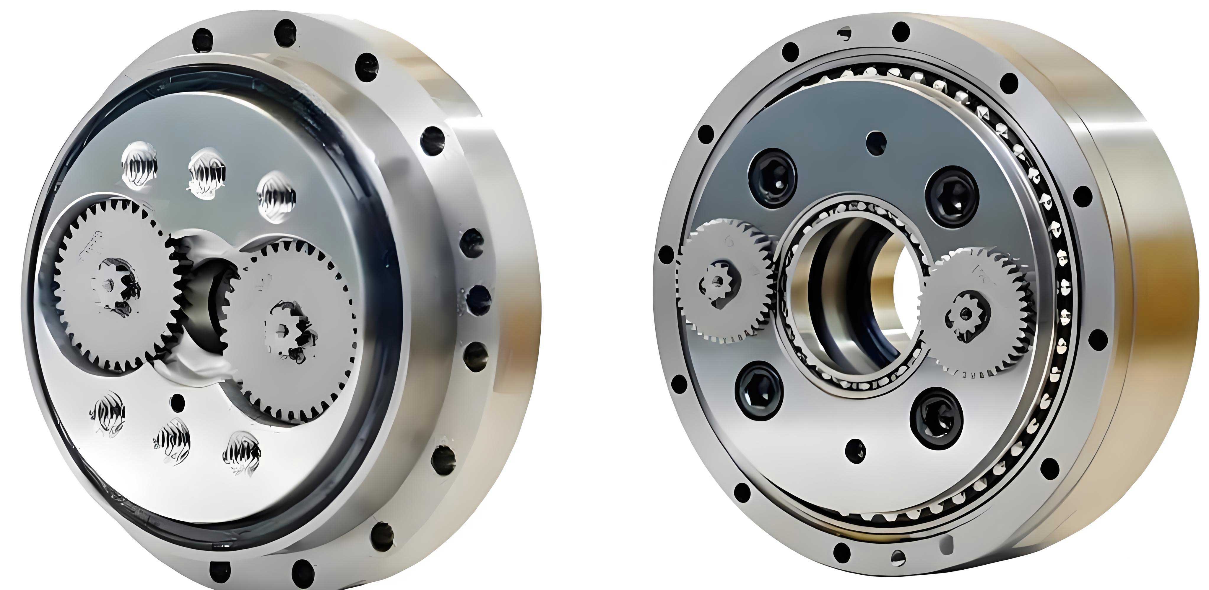
To understand the vibration behavior of the RV reducer, we first derive the theoretical vibration frequencies based on its kinematic parameters. The key frequencies include those associated with shaft rotations, gear meshing, and component motions. Let \( n_0 \) be the output speed in rpm, \( R \) the transmission ratio, and \( z_1, z_2, z_3, z_4 \) the tooth numbers of the input gear, planetary gear, cycloid gear, and pin housing, respectively. The fundamental frequencies are calculated as follows:
Input shaft frequency: $$f_1 = \frac{n_0 R}{60}$$
Output shaft characteristic frequency: $$f_0 = \frac{n_0}{60}$$
Planetary gear and crankshaft auto-rotation frequency: $$f_2 = \frac{z_1 z_2 (z_3 – z_4)}{(z_1 + z_2 z_4)} f_1$$
Planetary gear and crankshaft revolution frequency: $$f_3 = \frac{z_1}{z_1 + z_2 z_4} f_1$$
Cycloid gear auto-rotation frequency: $$f_4 = \frac{z_1}{z_1 + z_2 z_4} f_1$$
Cycloid gear revolution frequency: $$f_5 = \frac{z_1 z_4 (z_3 – z_4)}{(z_1 + z_2 z_4)} f_1$$
Planetary gear meshing frequency: $$f_{1c} = \frac{z_1 z_2 z_4}{z_1 + z_2 z_4} f_1$$
Cycloid gear meshing frequency: $$f_{4c} = \frac{z_1 z_3 z_4}{z_1 + z_2 z_4} f_1$$
For our experimental RV reducer model 190BX, the parameters are as listed in Table 1. These values are used to compute theoretical frequencies under various operating conditions.
| Parameter | Symbol | Value |
|---|---|---|
| Transmission Ratio | \( R \) | 121 |
| Input Gear Teeth | \( z_1 \) | 12 |
| Planetary Gear Teeth | \( z_2 \) | 36 |
| Cycloid Gear Teeth | \( z_3 \) | 39 |
| Pin Housing Teeth | \( z_4 \) | 40 |
We constructed a wireless torsional vibration test bench to capture acceleration signals from the RV reducer during operation. The setup includes a servo motor connected to the RV reducer’s input shaft, with the reducer’s pin housing fixed via a flange. A wireless acceleration sensor (model RNT301, range ±2g) was adhesively attached to the edge of the output flange in the tangential direction to measure torsional vibrations. The sampling frequency was set to 4000 Hz to ensure accurate signal acquisition. Tests were conducted on both superior and inferior RV reducer samples, identified based on empirical quality assessments. Each sample was run under no-load conditions at motor speeds of 1500, 2000, and 2500 rpm, in both forward and reverse directions. Multiple data sets were collected for consistency, and signals were preprocessed through mean removal and filtering.
The time-domain acceleration signals revealed differences in vibration magnitude between superior and inferior RV reducers. To quantify this, we computed the root mean square (RMS) values for each signal. For a discrete signal \({x_i}\) of length \(N\), the RMS is defined as:
$$X_{\text{RMS}} = \sqrt{\frac{1}{N} \sum_{i=1}^{N} x_i^2}$$
The computed RMS values for various operating conditions are summarized in Table 2. It is evident that inferior RV reducers exhibit significantly higher vibration levels compared to superior ones, indicating potential faults or manufacturing defects.
| Speed (rpm) | Sample Quality | Sample 1 RMS (g) | Sample 2 RMS (g) | Sample 3 RMS (g) | Average RMS (g) |
|---|---|---|---|---|---|
| 1500 | Superior | 0.0943 | 0.0921 | 0.0905 | 0.0923 |
| Inferior | 0.1636 | 0.1626 | 0.1734 | 0.1665 | |
| 2000 | Superior | 0.1899 | 0.1685 | 0.1584 | 0.1723 |
| Inferior | 0.2538 | 0.2620 | 0.2537 | 0.2565 | |
| 2500 | Superior | 0.1792 | 0.1719 | 0.1881 | 0.1797 |
| Inferior | 0.3465 | 0.3595 | 0.3661 | 0.3574 |
While time-domain analysis provides insights into vibration intensity, frequency-domain analysis is crucial for identifying specific vibration sources. However, due to the complexity of the RV reducer’s vibration signals, traditional Fourier analysis often fails to separate overlapping frequency components. To address this, we employed Variational Mode Decomposition (VMD), an adaptive signal processing technique that decomposes a signal into intrinsic mode functions (IMFs) with specific center frequencies and limited bandwidths. VMD solves a constrained variational problem to minimize the sum of bandwidths of all IMFs. The formulation is as follows:
$$\min_{\{u_k\},\{\omega_k\}} \left\{ \sum_k \left\| \partial_t \left[ \left( \delta(t) + \frac{j}{\pi t} \right) * u_k(t) \right] e^{-j\omega_k t} \right\|_2^2 \right\}$$
$$\text{subject to} \quad \sum_k u_k = f$$
where \(u_k\) are the IMFs, \(f\) is the original signal, \(\omega_k\) are the center frequencies, \(\delta(t)\) is the Dirac delta function, \(j\) is the imaginary unit, and \(\partial_t\) denotes the partial derivative with respect to time. To solve this, we introduce a quadratic penalty term \(\alpha\) and Lagrangian multiplier \(\lambda\), leading to the augmented Lagrangian:
$$\mathcal{L}(u_k,\omega_k,\lambda) = \alpha \sum_k \left\| \partial_t \left[ \left( \delta(t) + \frac{j}{\pi t} \right) * u_k(t) \right] e^{-j\omega_k t} \right\|_2^2 + \left\| f(t) – \sum_k u_k(t) \right\|_2^2 + \left\langle \lambda(t), f(t) – \sum_k u_k(t) \right\rangle$$
The solution is obtained iteratively using the alternating direction method of multipliers (ADMM). The update equations for \(u_k\) and \(\omega_k\) are:
$$u_k^{n+1}(\omega) = \frac{f(\omega) – \sum_{i \neq k} u_i(\omega) + \frac{\lambda(\omega)}{2}}{1 + 2\alpha (\omega – \omega_k)^2}$$
$$\omega_k^{n+1} = \frac{\int_0^\infty \omega |u_k(\omega)|^2 d\omega}{\int_0^\infty |u_k(\omega)|^2 d\omega}$$
Iterations continue until convergence, determined by a tolerance criterion. In our analysis, we applied VMD to torsional vibration signals from both superior and inferior RV reducers at 2500 rpm. Based on the theoretical frequency range (0-600 Hz), we set the number of modes \(N’ = 20\) to avoid over-decomposition or under-decomposition. The resulting IMFs were then analyzed via Fast Fourier Transform (FFT) to obtain their frequency spectra.
The VMD decomposition successfully extracted IMFs corresponding to key vibration frequencies of the RV reducer. For instance, IMF components from superior and inferior samples showed peaks at frequencies matching theoretical calculations. A comparison between theoretical and actual frequencies for the 190BX RV reducer at 2500 rpm is presented in Table 3. The close agreement validates the effectiveness of VMD in isolating relevant vibration modes.
| Frequency Type | Theoretical Frequency (Hz) | Actual Frequency (Hz) | Normalized Error (%) |
|---|---|---|---|
| Input Shaft Frequency \(f_1\) | 41.67 | 41.01 | 1.58 |
| Planetary Gear & Crankshaft Auto-rotation \(f_2\) | 13.77 | 13.67 | 0.72 |
| Cycloid Gear Revolution \(f_5\) | 13.77 | 13.67 | 0.72 |
| Planetary Gear Meshing \(f_{1c}\) | 495.87 | 498.05 | 0.44 |
| Cycloid Gear Meshing \(f_{4c}\) | 537.19 | 539.06 | 0.35 |
Further analysis focused on the IMFs containing low-frequency components, particularly around 13.67 Hz, which corresponds to \(f_2\) and \(f_5\). The spectral amplitudes at this frequency were compared between superior and inferior RV reducers. As shown in Table 4, inferior samples exhibited significantly higher amplitudes, indicating abnormal vibrations linked to planetary gear and crankshaft auto-rotation or cycloid gear revolution. This suggests manufacturing defects in these components, such as machining errors or assembly inaccuracies.
| Speed (rpm) | Sample Quality | Amplitude at 13.67 Hz (g) | Normalized Amplitude (Relative to Superior) |
|---|---|---|---|
| 1500 | Superior | 0.0042 | 1.00 |
| Inferior | 0.0285 | 6.79 | |
| 2000 | Superior | 0.0051 | 1.00 |
| Inferior | 0.0357 | 7.00 | |
| 2500 | Superior | 0.0073 | 1.00 |
| Inferior | 0.0467 | 6.40 |
To delve deeper, we examined the harmonic frequencies present in the IMFs. For example, higher-order harmonics of the input shaft frequency were observed, such as \(2f_1\) and \(3f_1\), which can be attributed to nonlinear effects or imbalances in the RV reducer. The VMD method effectively separated these harmonics, allowing for a comprehensive frequency analysis. The overall vibration energy distribution across IMFs was also computed using the following energy metric for each IMF \(u_k\):
$$E_k = \int_{-\infty}^{\infty} |u_k(t)|^2 dt$$
The relative energy contributions for key IMFs are summarized in Table 5. Notably, inferior RV reducers showed higher energy in IMFs associated with meshing frequencies and low-frequency components, corroborating the presence of faults.
| IMF Component | Center Frequency (Hz) | Superior RV Reducer Energy (%) | Inferior RV Reducer Energy (%) |
|---|---|---|---|
| IMF1 (Low-frequency) | 6.84 | 2.1 | 3.5 |
| IMF2 (13.67 Hz) | 13.67 | 5.3 | 15.8 |
| IMF3 (41.01 Hz) | 41.01 | 8.7 | 9.2 |
| IMF4 (83.98 Hz) | 83.98 | 7.5 | 8.1 |
| IMF5 (125.00 Hz) | 125.00 | 6.9 | 7.4 |
| IMF6 (498.05 Hz) | 498.05 | 22.4 | 25.6 |
| IMF7 (539.06 Hz) | 539.06 | 24.8 | 26.3 |
| Other IMFs | >600 Hz | 22.3 | 14.1 |
The robustness of the VMD approach was tested under different operational conditions, including varying speeds and directions. In all cases, the decomposition consistently identified the same set of characteristic frequencies, demonstrating its reliability for RV reducer vibration analysis. Additionally, we compared VMD with other methods like Empirical Mode Decomposition (EMD) and found that VMD provided better mode separation and less mode mixing, thanks to its rigorous mathematical formulation.
Based on the findings, we conclude that the abnormal vibrations in inferior RV reducers are primarily excited by the auto-rotation of planetary gears and crankshafts or the revolution of cycloid gears. This is likely due to machining errors in these components, such as tooth profile deviations or eccentricities. The VMD method proved instrumental in isolating these fault-related frequencies, offering a powerful tool for quality control and predictive maintenance of RV reducers. Future work could involve integrating machine learning algorithms with VMD for automated fault classification and real-time monitoring.
In summary, this study underscores the importance of advanced signal processing in enhancing the performance and reliability of RV reducers. By leveraging VMD, we can accurately diagnose vibration issues, leading to improvements in manufacturing processes and product quality. The methodologies developed here are applicable not only to RV reducers but also to other precision transmission systems in robotics and industrial machinery.