
The pursuit of precision and reliability in robotic and high-precision automation drives continuous innovation in core components. Among these, the RV (Rotate Vector) reducer stands out as a critical transmission element. Renowned for its exceptional features—high positioning accuracy, substantial reduction ratio, compact structure, and excellent torsional stiffness—the RV reducer is indispensable in applications such as industrial robot joints, CNC machine tools, and precision medical equipment. However, the manufacturing and assembly quality of RV reducers directly influence these performance metrics. Due to numerous influencing factors and inherent process variations, achieving consistent assembly quality remains a significant industrial challenge. An unstable assembly process leads to high rework rates, increased costs, and delivery delays. Therefore, developing an effective method to predict key performance indicators (KPIs) before final assembly is crucial. This enables intelligent part selection and matching, moving away from traditional trial-and-error approaches and significantly enhancing production efficiency and product quality.
This article focuses on predicting the transmission error, a paramount KPI for RV reducers. Transmission error, defined as the deviation between the actual and theoretical output position for a given input, directly impacts operational precision, vibration, noise, and service life. We propose a robust prediction model based on a BP (Backpropagation) neural network, further enhanced by the Sparrow Search Algorithm (SSA). By selecting key dimensional parameters of critical components as inputs, the model learns the complex, non-linear relationship between these parameters and the resulting transmission error of the assembled RV reducer.
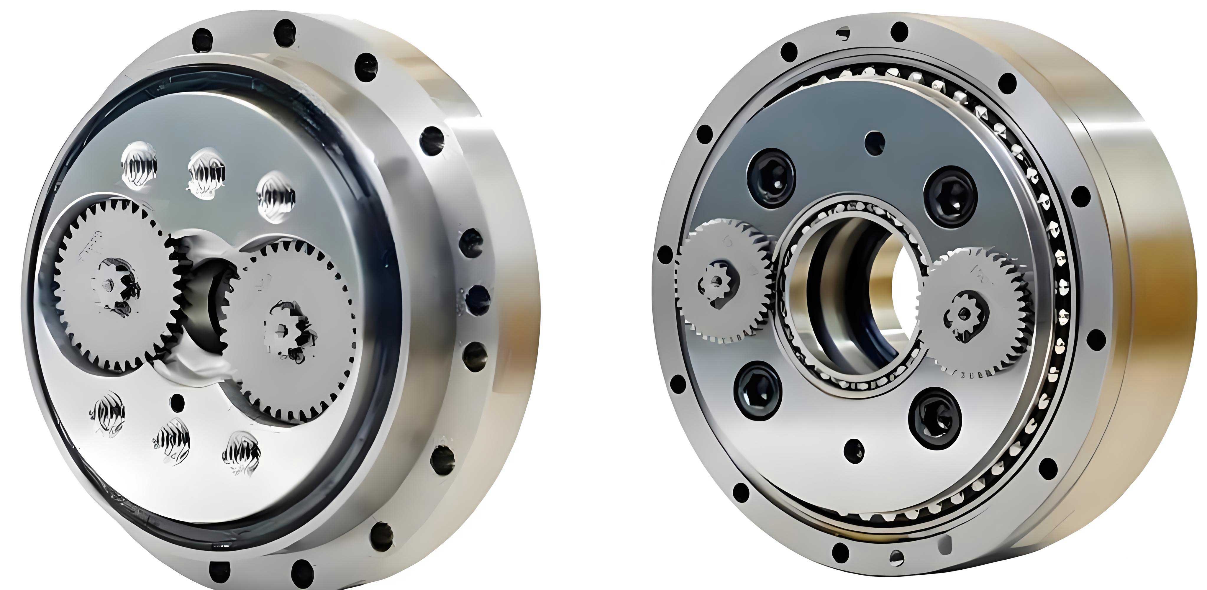
Analysis of Quality Influencing Factors for RV Reducers
The RV reducer is a two-stage precision transmission device. The first stage consists of a planetary gear train, and the second stage is a cycloid-pin gear mechanism. The final output is derived from the cycloid disc motion transmitted through a crank shaft and a planet carrier. The interplay of dimensions across these components—cycloid disc, needle pins and shell, crank shaft eccentric journals, and planet carrier holes—collectively determines the final meshing quality and clearance state, thereby dictating the transmission error.
Key dimensional parameters identified as primary influencers include:
- Cycloid disc parameters: Span measurement over pins (a critical indirect measure of tooth profile geometry), and the diameters of its mounting holes.
- Crank shaft parameters: Diameters of the eccentric journals and associated friction torque measurements.
- Pin gear shell parameter: Root circle diameter.
- Planet carrier parameters: Diameters of the crank shaft bearing mounting holes.
- Pin parameters: Diameter and associated friction torque.
Prior research has consistently highlighted that errors in the cycloid tooth profile, often reflected in the span measurement, have the most pronounced effect on the output angle error of the transmission. In practical manufacturing, the cycloid disc is among the most challenging components to produce, leading to unavoidable variations in its key parameters. Consequently, assembly often requires selective fitting of other components based on the actual dimensions of the cycloid disc. The relationship between these many parameters and the final transmission error is highly complex and non-linear, making empirical selection inefficient. This complexity necessitates an intelligent modeling approach to capture these relationships for accurate pre-assembly prediction of the RV reducer‘s performance.
Mathematical Foundation: The BP Neural Network
The BP neural network is a classic multi-layer feedforward network trained by error backpropagation. Its structure typically includes an input layer, one or more hidden layers, and an output layer. The learning process involves a forward pass to compute the output and a backward pass to adjust the weights and biases (thresholds) based on the prediction error.
Let us define the following for a network with \(n\) inputs, \(p\) hidden neurons, and \(q\) outputs:
$$ X = [x_1, x_2, …, x_n]^T \quad \text{(Input vector)} $$
$$ Y = [y_1, y_2, …, y_q]^T \quad \text{(Actual output vector)} $$
$$ O = [o_1, o_2, …, o_q]^T \quad \text{(Target output vector)} $$
$$ B = [b_1, b_2, …, b_p]^T \quad \text{(Hidden layer output vector)} $$
$$ W_j = [w_{j1}, w_{j2}, …, w_{jn}]^T, \quad j=1,2,…,p \quad \text{(Weights from input to hidden layer)} $$
$$ V_k = [v_{k1}, v_{k2}, …, v_{kp}]^T, \quad k=1,2,…,q \quad \text{(Weights from hidden to output layer)} $$
$$ \theta_j, \theta_k \quad \text{(Biases for hidden and output layers, respectively)} $$
The forward propagation calculation is as follows:
- Input and output for the hidden layer:
$$ s_j = \sum_{i=1}^{n} w_{ji} x_i – \theta_j, \quad j=1,2,…,p $$
$$ b_j = f(s_j) = \frac{1}{1 + e^{-s_j}} \quad \text{(using sigmoid activation)} $$ - Input and output for the output layer:
$$ s_k = \sum_{j=1}^{p} v_{kj} b_j – \theta_k, \quad k=1,2,…,q $$
$$ y_k = g(s_k) \quad \text{(often linear activation for regression)} $$
The backward error propagation and parameter update rules are:
- Calculate the error terms:
For the output layer: $$ \delta_k^o = (o_k – y_k) \cdot g'(s_k) $$
For the hidden layer: $$ \delta_j^h = \left( \sum_{k=1}^{q} \delta_k^o v_{kj} \right) \cdot f'(s_j) $$ - Update weights and biases (using learning rates \(\alpha\) and \(\beta\)):
$$ \Delta v_{kj} = \alpha \cdot \delta_k^o \cdot b_j, \quad \Delta \theta_k = \alpha \cdot \delta_k^o $$
$$ \Delta w_{ji} = \beta \cdot \delta_j^h \cdot x_i, \quad \Delta \theta_j = \beta \cdot \delta_j^h $$
The standard BP algorithm is sensitive to the initial random values of \(W\) and \(V\), which can lead to convergence to local minima and unstable prediction performance. This limitation motivates the use of a metaheuristic optimization algorithm for superior initialization and training.
Enhanced Optimization: The Sparrow Search Algorithm (SSA)
The Sparrow Search Algorithm is a novel population-based metaheuristic inspired by the foraging and anti-predation behaviors of sparrow flocks. The population is divided into three roles: producers (discoverers), scroungers (followers), and scouts.
For an optimization problem with \(d\) dimensions, the position of the \(i\)-th sparrow in the population is represented as:
$$ X_i = [x_{i,1}, x_{i,2}, …, x_{i,d}] $$
The fitness value \(f(X_i)\) evaluates the quality of the solution, which in our context is the prediction error of the neural network with the corresponding weight/bias set.
The position update rules for each role during iteration \(t\) are defined below, where \(iter_{max}\) is the maximum number of iterations, \(\alpha \in (0,1]\), \(R_2 \in [0,1]\) is an alarm value, \(ST \in [0.5,1]\) is a safety threshold, \(Q\) is a random number from a normal distribution, and \(L\) is a \(1 \times d\) matrix of ones.
1. Producer Update: Producers search for food sources. Their positions are updated as:
$$ X_{i,j}^{t+1} = \begin{cases}
X_{i,j}^{t} \cdot \exp\left(-\frac{i}{\alpha \cdot iter_{max}}\right), & \text{if } R_2 < ST \text{ (safe)} \\
X_{i,j}^{t} + Q \cdot L, & \text{if } R_2 \ge ST \text{ (danger)}
\end{cases} $$
where \(j=1,2,…,d\).
2. Scrounger Update: Scroungers follow the producers to feed. Their positions are updated as:
$$ X_{i,j}^{t+1} = \begin{cases}
Q \cdot \exp\left(\frac{X_{worst}^{t} – X_{i,j}^{t}}{i^2}\right), & \text{if } i > n/2 \\
X_{P}^{t+1} + |X_{i,j}^{t} – X_{P}^{t+1}| \cdot A^{+} \cdot L, & \text{otherwise}
\end{cases} $$
Here, \(X_P\) is the best producer’s position, \(X_{worst}\) is the global worst position, \(A\) is a \(1 \times d\) matrix with randomly assigned 1 or -1, and \(A^{+} = A^T (A A^T)^{-1}\).
3. Scout Update: Scouts (a portion of the population) remain vigilant for danger. If a threat is detected, they drive the flock to safety. Their position update is:
$$ X_{i,j}^{t+1} = \begin{cases}
X_{best}^{t} + \beta \cdot |X_{i,j}^{t} – X_{best}^{t}|, & \text{if } f_i > f_g \\
X_{i,j}^{t} + K \cdot \left( \frac{|X_{i,j}^{t} – X_{worst}^{t}|}{(f_i – f_w) + \epsilon} \right), & \text{if } f_i = f_g
\end{cases} $$
where \(X_{best}\) is the current global best position; \(f_i, f_g, f_w\) are the current individual, global best, and global worst fitness values, respectively; \(\beta\) and \(K\) are step control parameters; and \(\epsilon\) is a small constant to avoid division by zero.
The Integrated SSA-BP Prediction Model for RV Reducers
The integration of SSA with the BP neural network aims to optimize the initial weights and biases, thereby guiding the network toward a superior global optimum and improving its prediction accuracy and stability. The steps of the SSA-BP algorithm are as follows:
- Initialization: Define the BP network structure (input, hidden, output nodes). Initialize the SSA parameters: population size \(n\), maximum iterations \(iter_{max}\), proportions of producers and scouts, \(ST\), etc. The optimization variables (dimension \(d\)) are the flattened vector containing all weights \(W, V\) and biases \(\theta\) of the BP network.
- Fitness Evaluation: For each sparrow (each set of network parameters), construct the corresponding BP network. Use it to predict on both the training and validation datasets. The fitness value is calculated as the sum of the Mean Squared Error (MSE) on both sets to balance learning and generalization:
$$ fitness = argmin( MSE_{train} + MSE_{val} ) $$
$$ MSE = \frac{1}{N} \sum_{i=1}^{N} (y_i^{true} – y_i^{pred})^2 $$ - SSA Iteration: Perform the SSA position updates for producers, scroungers, and scouts as per the equations above, based on the calculated fitness values. This process evolves the population of potential network parameter sets.
- Termination and Deployment: After reaching \(iter_{max}\), select the sparrow with the best fitness (lowest combined MSE). Its position vector is decoded into the optimal initial weights and biases for the BP network. This optimized network is then trained briefly with the standard BP algorithm on the full training set to fine-tune the solution. The final model is used for predicting the transmission error of the RV reducer.
Case Study: Application and Results for an RV Reducer Model
1. Variable Selection and Data Preparation
A specific model of RV reducer (42N-126 type) was selected for this study. Fifteen (15) key dimensional and assembly parameters were identified as input features \(x_1\) to \(x_{15}\). The output target \(y\) is the measured transmission error. A dataset of 114 complete assemblies was collected from the production line.
| Symbol | Parameter Description | Symbol | Parameter Description |
|---|---|---|---|
| x1 | Cycloid Disc Span Measurement | x9 | Friction Torque (Eccentric 3) |
| x2 | Cycloid Disc Hole 1 Diameter | x10 | Pin Gear Shell Root Circle Diameter |
| x3 | Cycloid Disc Hole 2 Diameter | x11 | Planet Carrier Hole 1 Diameter |
| x4 | Crank Shaft Eccentric 1 Diameter | x12 | Planet Carrier Hole 2 Diameter |
| x5 | Friction Torque (Eccentric 1) | x13 | Ball Bearing Friction Torque |
| x6 | Crank Shaft Eccentric 2 Diameter | x14 | Pin Diameter |
| x7 | Friction Torque (Eccentric 2) | x15 | Pin Friction Torque |
| x8 | Crank Shaft Eccentric 3 Diameter | y | Transmission Error |
The data was preprocessed: outliers were removed, and all features were normalized to the range [-1, 1] using min-max scaling to accelerate network convergence:
$$ x^{*} = (y_{max} – y_{min}) \cdot \frac{x – x_{min}}{x_{max} – x_{min}} + y_{min} $$
where \(y_{max}=1\) and \(y_{min}=-1\). The dataset was split into 88 samples for training and 26 samples for independent testing.
| Sample | x1 | x2 | x3 | x4 | x5 | … | y (Target) |
|---|---|---|---|---|---|---|---|
| 1 | -0.7575 | -0.5682 | 0.2000 | 0.9831 | -1.0000 | … | -0.0833 |
| 2 | -0.8623 | -0.7045 | -0.6941 | 0.9812 | 0.6000 | … | 0.4167 |
| 3 | -0.7827 | -0.2422 | 0.4353 | 0.9673 | -0.2000 | … | 0.5833 |
| 4 | -0.8021 | -0.3864 | 0.2706 | 0.9871 | -0.6000 | … | 0.1677 |
| 5 | -0.7905 | -0.5227 | 0.1294 | 0.9841 | -1.0000 | … | 0.0000 |
2. Model Configuration and Parameter Setting
The BP network structure was determined as 15-10-1 (15 inputs, 10 hidden neurons, 1 output). The hidden layer uses a sigmoid activation function, while the output layer uses a linear function. The SSA parameters were set as: population size = 20, \(iter_{max} = 20\), \(ST = 0.6\), producer ratio = 0.7, scout ratio = 0.2. The search boundaries for all weights and biases were set to [-5, 5].
3. Results and Comparative Analysis
The performance of the proposed SSA-BP model was compared against a standard BP neural network model with random initialization. The convergence curve of the SSA during the optimization of the BP network’s parameters shows a steady decrease in the best fitness value (combined MSE), indicating effective search behavior.
The prediction results on the independent test set are summarized below. The SSA-BP model’s predictions are significantly closer to the actual measured transmission error values compared to the standard BP model.
| Prediction Model | Mean Squared Error (MSE) on Test Set | Key Observation |
|---|---|---|
| Standard BP Neural Network | 0.025146 | Higher error, greater prediction variance. |
| SSA-Optimized BP Neural Network | 0.008825 | ~65% lower MSE, more stable and accurate predictions. |
The error distribution for the SSA-BP model is markedly tighter around zero compared to the standard BP model. This demonstrates that the SSA optimization effectively mitigates the issue of converging to poor local minima, leading to a more reliable and precise model for forecasting the performance of the RV reducer based on component dimensions.
Conclusion and Outlook
This work successfully developed and applied an SSA-optimized BP neural network model for predicting the transmission error of RV reducers prior to final assembly. By utilizing key dimensional parameters of critical components as inputs, the model effectively captures the complex, non-linear relationships governing the assembly quality. The integration of the Sparrow Search Algorithm provides a systematic method to initialize and optimize the neural network’s parameters, resulting in a model with superior prediction accuracy and stability compared to the traditional BP approach. The significant reduction in prediction error (MSE) validates the efficacy of the proposed method.
This intelligent prediction model provides a practical tool for the assembly line. It enables data-driven selective assembly, where components can be chosen to pair together to achieve a desired transmission error range, thereby reducing reliance on trial-and-error, minimizing rework, improving first-pass yield, and lowering production costs for high-precision RV reducer systems.
Future work will focus on expanding the model’s scope. The current analysis primarily considers dimensional parameters (“machine” and “material” factors). A more comprehensive model could integrate additional influential factors from the “Man, Method, and Environment” categories, such as operator skill, assembly sequence and torque, and ambient temperature. Furthermore, exploring other advanced metaheuristic algorithms and deep learning architectures may yield further improvements in prediction capability and robustness for the next generation of precision transmission systems.