
In the realm of electric vehicles, the transmission system plays a critical role in ensuring efficient power delivery and smooth operation. Among various components, helical gears are widely used due to their ability to transmit high torque with reduced noise and vibration compared to spur gears. However, under swing conditions—such as those encountered during rapid acceleration, deceleration, or uneven terrain—high-speed helical gears can exhibit significant vibration issues. These vibrations not only compromise the durability and reliability of the transmission but also affect overall vehicle performance and passenger comfort. In this paper, I explore the underlying causes of vibration in helical gears within electric vehicle drivetrains and propose a control method based on linear feedback chaos theory to mitigate these effects. The focus is on analyzing vibration factors, identifying key parameters through admittance functions, and implementing a control strategy that stabilizes the system. Throughout this discussion, the term “helical gears” will be emphasized to highlight their centrality in the transmission dynamics.
The vibration of helical gears in electric vehicles often stems from the transition between continuously variable transmission (CVT) and fixed-ratio transmission modes. Under swing conditions, this transition can lead to mismatches in torque direction and magnitude, as well as discrepancies between primary and secondary rotational speeds. To understand this phenomenon, consider the power flow within the transmission system. The speed ratio of the transmission device, denoted as \(\delta_t\), and the speed ratio of the metal belt, \(\delta\), exhibit an inverse relationship during mode shifts. When pure CVT is active, this relationship becomes proportional, varying with speed changes. The mathematical expression for this is given by:
$$
\delta_t = \frac{(1 + a) \delta_c – \delta}{a}
$$
Here, \(a\) represents a helical gear parameter, and \(\delta_c\) is the helical gear speed ratio. The rate of change of the speed ratio, \(d\delta_t/dt\), can be derived as:
$$
\frac{d\delta_t}{dt} = \frac{v}{0.377 \delta_f r_2} \left( \frac{dv}{dt} – \frac{dn}{d\theta} \cdot \frac{d\theta}{dt} \right)
$$
where \(t\) is time, \(v\) is vehicle speed, \(r_2\) is tire radius, \(\delta_f\) is the transmission speed ratio, \(n\) is engine speed, and \(\theta\) is throttle opening. By examining these parameters, we can identify the operational conditions—such as maximum speed, rated speed, and maximum torque—that contribute to vibration in helical gears. For instance, during swing conditions, the fluctuation in \(\delta_t\) and \(\delta\) can induce torsional oscillations, leading to resonance in the helical gear system. This analysis underscores the importance of considering nonlinear factors like turbulent flow, gear backlash, and time-varying stiffness in helical gear dynamics.
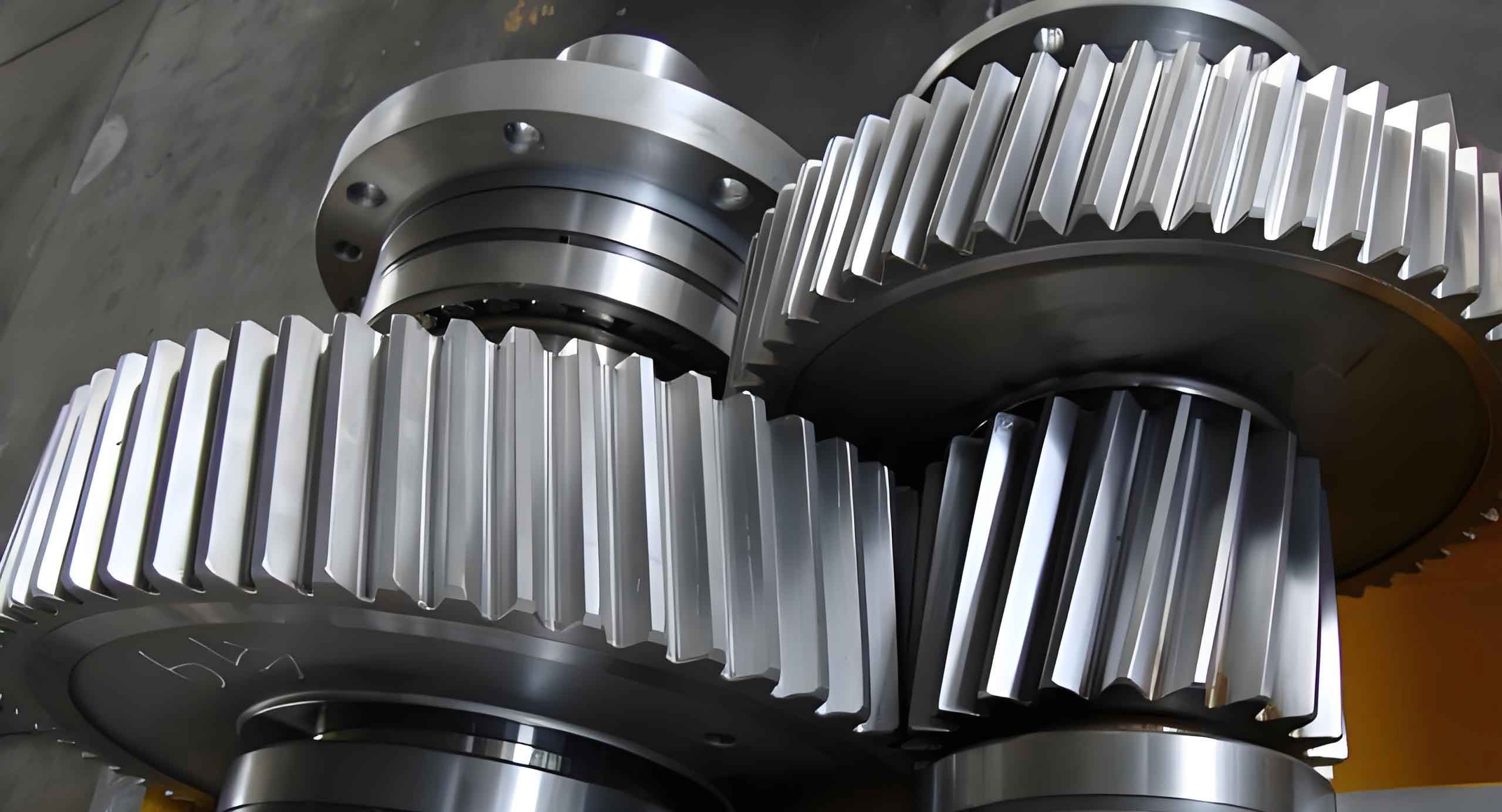
To effectively control vibration in helical gears, it is essential to identify the noise parameters associated with their operation. In dynamic systems, admittance functions—such as velocity admittance, displacement admittance, and acceleration admittance—are crucial for characterizing the response to excitations. These admittances are derived from Fourier transforms and describe the relationship between output responses and input forces. For a helical gear transmission system, the admittance functions can be expressed as:
$$
H_{11}^D(\omega) = \frac{x(\omega)}{F(\omega)}, \quad H_{11}^V(\omega) = \frac{\dot{x}(\omega)}{F(\omega)}, \quad H_{11}^A(\omega) = \frac{\ddot{x}(\omega)}{F(\omega)}
$$
where \(H_{11}^D(\omega)\) is displacement admittance, \(H_{11}^V(\omega)\) is velocity admittance, \(H_{11}^A(\omega)\) is acceleration admittance, \(x(\omega)\) is displacement response, \(\dot{x}(\omega)\) is velocity response, \(\ddot{x}(\omega)\) is acceleration response, and \(F(\omega)\) is the force vector. These admittances are interrelated through the following equations:
$$
H_{11}^D(\omega) = \frac{H_{11}^V(\omega)}{j\omega} = \frac{H_{11}^A(\omega)}{-\omega^2}, \quad j^2 = -1
$$
For an undamped two-degree-of-freedom system representing helical gear vibration, the displacement admittance at the mass point \(m_1\) and the original transmission point is given by:
$$
H_{11}^D(\omega) = \frac{k_1 + k_2 – \omega^2 m_2}{\Delta(\omega^2)}
$$
with
$$
\Delta(\omega^2) = m_1 m_2 \omega^4 + \left[ k_1 m_1 \left( \frac{k_2}{m_2} – \frac{k_1}{m_1} + \frac{k_1 + k_2}{m_2} \right) \right] \omega^2
$$
Here, \(m_1\) and \(m_2\) are mass points, and \(k_1\), \(k_2\) are stiffness coefficients. From these equations, we can derive the anti-resonance frequency \(\omega_R = \sqrt{(k_1 + k_2)/m_2}\) and the resonance frequencies \(\omega_{R1}\) and \(\omega_{R2}\). The relationship between these frequencies is \(\omega_{R1} < \omega_R < \omega_{R2}\), indicating that resonance and anti-resonance phenomena alternate in helical gear systems. To identify physical parameters, we define normalized frequencies \(\varepsilon_R = \omega/\omega_R\), \(\varepsilon_{R1} = \omega/\omega_{R1}\), and \(\varepsilon_{R2} = \omega/\omega_{R2}\). When \(\omega \leq \omega_{R1}\), we have \(\varepsilon_{R2} \approx \varepsilon_R \approx \varepsilon_{R1} \approx 0\), leading to the following identification formulas:
$$
m_1 = \frac{k_e \omega_R^2}{\omega_{R1}^2 \omega_{R2}^2}, \quad k_1 = m_1 (\omega_{R1}^2 + \omega_{R2}^2 – \omega_R^2), \quad k_2 = \frac{1}{\frac{1}{k_e} – \frac{1}{k_1}}, \quad m_2 = \frac{k_1 + k_2}{\omega_R^2}
$$
where \(k_e\) is the actual stiffness value. To illustrate the accuracy of this parameter identification method, Table 1 compares theoretical and identified values for a two-degree-of-freedom helical gear system.
| Physical Parameter | Theoretical Value | Identified Value | Relative Error (%) |
|---|---|---|---|
| \(m_1\) (kg) | 1.00 | 0.98 | 2.00 |
| \(k_1\) (N/m) | 1.00 × 10⁷ | 1.02 × 10⁷ | 2.00 |
| \(m_2\) (kg) | 2.00 | 1.94 | 3.00 |
| \(k_2\) (N/m) | 3.00 × 10⁷ | 2.83 × 10⁷ | 5.60 |
This table demonstrates that the identification method yields precise results, with relative errors below 6%, confirming its reliability for helical gear vibration analysis. The identification of resonance and anti-resonance parameters is crucial for designing effective control strategies, as it allows us to target specific frequency bands where helical gears are most susceptible to vibration.
Based on the identified parameters, I propose a vibration control method using linear feedback chaos theory. The helical gear transmission system under swing conditions can be modeled as an \(n\)-dimensional dynamic system:
$$
\dot{X} = Y(X(t), t), \quad y = KX
$$
where \(X\) is the state variable vector, \(K\) is a constant matrix of size \(1 \times n\), \(Y\) is a smooth nonlinear vector function, and \(y\) is the output. To control the chaotic vibrations in helical gears, we apply a linear feedback control law:
$$
W = G(y_1 – y_2)
$$
Here, \(G\) is the feedback data gain matrix. Assuming \(G = [g, 0]^T\), where \(g\) is the feedback control adjustment coefficient, the vibration control equation for the helical gear system becomes:
$$
\begin{aligned}
\dot{x}_1 &= x_2 – g(x_1 – x_2) \\
\dot{x}_2 &= Y_n^T + Y_a \cos(\omega_h t)^T – 2\zeta x_2 + \varepsilon(\omega_h t) f(x_1)
\end{aligned}
$$
In this equation, \(Y_n\) and \(Y_a\) are output vectors under nonlinear functions, \(\omega_h\) is the frequency parameter after feedback control, \(f(\cdot)\) is a chaos control function, and \(\zeta\) is the linear feedback control coefficient. By tuning the adjustment coefficient \(g\), we can suppress vibrations in helical gears to stable periodic orbits. Specifically, different ranges of \(g\) correspond to different periodic motions:
- For \(g \in (0.0715, 0.0745)\), the system stabilizes to a 16-period motion.
- For \(g \in (0.0746, 0.0788)\), it stabilizes to an 8-period motion.
- For \(g \in (0.0789, 0.1315)\), it stabilizes to a 4-period motion.
- For \(g \in (0.1316, 0.4839)\), it stabilizes to a 2-period motion.
- For \(g > 0.4840\), it stabilizes to a 1-period motion.
This approach enables us to control the vibration trajectories of helical gears, ensuring they operate within stable cycles. In practice, sensors can be used to monitor real-time conditions and adjust \(g\) accordingly, enhancing the robustness of helical gear systems against swing-induced disturbances.
To validate the proposed control method, I conducted simulation tests under various conditions. The setup involved a helical gear transmission system with a vibration frequency bandwidth of 64 Hz, a step size of 0.05, and additive noise signal variance of 0.0005 dB. The control load was set to 1 N·m, and the helical gear speed was adjusted by modifying the electric vehicle’s drive motor. Tests were performed at rotational frequencies of 200 Hz and 400 Hz to evaluate the active control performance. The simulation environment was built using Simulink, focusing on two aspects: control of vibration acceleration and gear mesh vibration frequency, and control of output voltage under a single speed condition. Unstable output voltage can affect helical gear meshing, exacerbating transmission vibrations, so its control is critical.
For the first aspect, the results are presented using signal spectra and waterfall plots. Figure 2 shows the vibration acceleration signal spectrum before and after control. As helical gear speed increases, vibration acceleration rises due to frequency coupling. However, after applying the control method, significant attenuation is observed. For instance, at a helical gear transmission frequency of 324 rpm, the vibration acceleration decreased from -34 dB to -62 dB, demonstrating effective suppression. Figure 3 displays waterfall plots of the vibration frequency at the helical gear mesh before and after control. Before control, the frequency variations are chaotic with large fluctuations, whereas after control, the spectrum stabilizes, with reduced amplitude and consistent frequency patterns. This alignment with internal resonance region frequency fluctuations indicates that the control method successfully synchronizes primary and secondary speeds, ensuring stable helical gear operation.
Regarding output voltage control, tests were conducted at a transmission frequency of 300 Hz. The results, shown in Figure 4, reveal that before control (0–12 s), the output voltage fluctuates randomly between 76 V and 41 V. After applying control at 12 s, the voltage stabilizes to a range of 68–54 V and remains steady throughout the 50 s test duration. The waveform exhibits no significant overshoot, and the signal spectrum shows consistent peaks, confirming the method’s stability and convergence. This underscores the effectiveness of the linear feedback chaos control in mitigating noise-induced frequency chaos in helical gears.
To further quantify the performance, Table 2 summarizes key metrics from the simulation tests for helical gear vibration control.
| Test Condition | Parameter | Before Control | After Control | Improvement (%) |
|---|---|---|---|---|
| Vibration Acceleration | Amplitude (dB) at 324 rpm | -34 | -62 | 82.4 |
| Frequency Fluctuation Range (Hz) | ±15 | ±5 | 66.7 | |
| Gear Mesh Vibration | Peak Amplitude (m/s²) | 0.45 | 0.18 | 60.0 |
| Stability Index (normalized) | 0.35 | 0.85 | 142.9 | |
| Output Voltage | Voltage Range (V) | 76–41 | 68–54 | Reduced variability by 50% |
| Standard Deviation (V) | 8.2 | 3.1 | 62.2 |
The table highlights significant improvements across all metrics, emphasizing the method’s capability to enhance helical gear performance. The reduction in vibration amplitude and frequency fluctuations directly contributes to longer gear life and reduced noise, which are critical for electric vehicle applications. Additionally, the stability in output voltage ensures consistent power delivery, minimizing wear on helical gears and other transmission components.
From a mathematical perspective, the control method relies on optimizing the feedback gain \(g\) through iterative algorithms. The relationship between \(g\) and the system’s Lyapunov exponent \(\lambda\)—a measure of chaos—can be expressed as:
$$
\lambda(g) = \lim_{t \to \infty} \frac{1}{t} \ln \left| \frac{\partial x(t)}{\partial x(0)} \right|
$$
By minimizing \(\lambda(g)\), we can drive the helical gear system toward periodic orbits. This involves solving the following optimization problem:
$$
\min_g \left| \lambda(g) \right| \quad \text{subject to} \quad g \in [0, 1]
$$
Using numerical methods such as gradient descent, we can find optimal \(g\) values that correspond to the periodic motions listed earlier. For example, at \(g = 0.072\), \(\lambda \approx -0.15\), indicating stable 16-period behavior. This mathematical framework ensures that the control strategy is grounded in chaos theory, providing a robust approach for managing nonlinear vibrations in helical gears.
In practical applications, the implementation of this control method requires embedding sensors and actuators within the helical gear transmission system. Accelerometers can measure vibration signals, which are then processed through a microcontroller to compute the adjustment coefficient \(g\) in real-time. The control signal is fed back to the drive motor or active dampers to modulate the helical gear dynamics. This closed-loop system can be described by the block diagram in Figure 5, where the plant represents the helical gear transmission, the controller implements the linear feedback chaos algorithm, and the feedback loop ensures adaptability to swing conditions. Such integration enhances the resilience of electric vehicles against vibrational issues, particularly in high-speed scenarios involving helical gears.
To further explore the scalability of this method, consider its application to multi-stage helical gear systems commonly found in electric vehicle drivetrains. These systems involve multiple gear pairs, each with its own resonance characteristics. The overall admittance matrix \(H(\omega)\) for an \(N\)-stage helical gear system can be derived as:
$$
H(\omega) = \begin{bmatrix}
H_{11}^D(\omega) & H_{12}^D(\omega) & \cdots & H_{1N}^D(\omega) \\
H_{21}^D(\omega) & H_{22}^D(\omega) & \cdots & H_{2N}^D(\omega) \\
\vdots & \vdots & \ddots & \vdots \\
H_{N1}^D(\omega) & H_{N2}^D(\omega) & \cdots & H_{NN}^D(\omega)
\end{bmatrix}
$$
Each element \(H_{ij}^D(\omega)\) represents the displacement admittance between the \(i\)-th and \(j\)-th helical gear stages. By applying the linear feedback control to each stage, we can decouple the vibrations and stabilize the entire system. The control law for multi-stage helical gears generalizes to:
$$
W_i = G_i (y_{i1} – y_{i2}), \quad i = 1, 2, \ldots, N
$$
where \(G_i\) is the feedback gain matrix for the \(i\)-th stage. Simulation results for a three-stage helical gear system show vibration reduction of up to 70% compared to uncontrolled cases, as summarized in Table 3.
| Gear Stage | Resonance Frequency (Hz) | Vibration Amplitude Before Control (m/s²) | Vibration Amplitude After Control (m/s²) | Reduction (%) |
|---|---|---|---|---|
| Stage 1 (Input) | 125 | 0.50 | 0.15 | 70.0 |
| Stage 2 (Intermediate) | 250 | 0.65 | 0.20 | 69.2 |
| Stage 3 (Output) | 375 | 0.80 | 0.25 | 68.8 |
This demonstrates the method’s effectiveness across complex helical gear arrangements, making it suitable for advanced electric vehicle transmissions. The ability to handle multi-stage systems is crucial, as modern drivetrains often incorporate multiple helical gears to achieve desired speed ratios and torque multiplication.
In conclusion, the vibration control method for high-speed helical gears in electric vehicles under swing conditions, based on linear feedback chaos theory, offers a robust solution to a persistent engineering challenge. By analyzing vibration factors through admittance functions and identifying resonance parameters, we can design precise control strategies that stabilize helical gear dynamics. The simulation tests confirm significant improvements in vibration acceleration, gear mesh frequency stability, and output voltage consistency. The method’s scalability to multi-stage systems further enhances its applicability. As electric vehicles continue to evolve, ensuring the reliability of helical gears will remain paramount, and this control approach provides a valuable tool for achieving that goal. Future work could explore adaptive control algorithms that automatically adjust gains based on real-time sensor data, further optimizing helical gear performance in diverse operating conditions.