
In this article, I present a complete virtual cutting method for spiral bevel gears, starting from geometric parameter calculation and proceeding through cutter modeling, Boolean cutting simulation, surface reconstruction, tooth-surface accuracy verification, and finite element contact analysis. My objective is to show how a spiral bevel gear pair can be modeled with high precision and how the resulting digital model can be used to study tooth contact behavior under load. The method is intended to support later optimization of transmission error, contact pattern correction, and dynamic performance evaluation of spiral bevel gear systems. I use a combination of analytical formulas, CAD-based cutting simulation, surface reconstruction, and finite element analysis to achieve this goal.
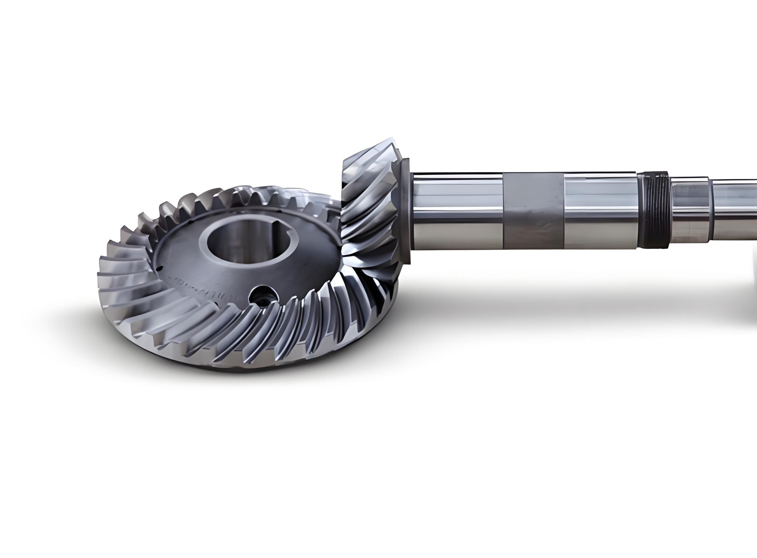
Spiral bevel gears are widely used in automotive, aerospace, mining, and heavy machinery transmissions because they offer a large overlap ratio, high transmission ratio, smooth operation, and low noise. As a key component of reducers and differentials, the performance, quality, and service life of a spiral bevel gear directly influence the economic and technical indicators of the entire product. Computer information technology has greatly improved the design, development, and manufacturing of spiral bevel gears. In the fields of spiral bevel gear simulation machining and finite element analysis, many researchers have made significant progress. Some have used finite element methods to study load distribution, actual contact ratio, and stress analysis. Others have proposed load-sharing formulas and investigated loaded transmission error. Still others have combined programming environments with CAD systems to simulate the CNC milling of spiral bevel gears. These developments show that simulation machining and finite element technology for spiral bevel gears are advancing rapidly, with continuously improving design accuracy and increasingly diversified design and analysis methods. In finite element analysis of spiral bevel gears, model accuracy has a decisive influence on the final results. Therefore, I focus on establishing a high-precision spiral bevel gear model and performing tooth-surface contact analysis.
1. Design Parameter Calculation for the Spiral Bevel Gear Blank
The blank of a spiral bevel gear mainly consists of the face cone, root cone, and central hub. Because the spiral bevel gear blank is a body of revolution, the problem of drawing the blank reduces to determining its two-dimensional cross-section. To define the shape of this cross-section, I need the pitch cone angle, face cone angle, and root cone angle. These parameters control the basic geometry of the spiral bevel gear and are essential for subsequent cutter positioning and cutting simulation.
The pitch cone angle is the angle between the pitch cone generatrix and the gear axis. For a pair of meshing spiral bevel gears, the sum of the pinion pitch cone angle and the wheel pitch cone angle equals the shaft angle. I calculate the wheel pitch cone angle and pinion pitch cone angle as follows:
$$ \delta_2 = \arctan\left(\frac{z_2 \sin \Sigma}{z_1 + z_2 \cos \Sigma}\right) $$
$$ \delta_1 = \Sigma – \delta_2 $$
Here, \(z_1\) is the number of pinion teeth, \(z_2\) is the number of wheel teeth, \(\Sigma\) is the shaft angle, \(\delta_1\) is the pinion pitch cone angle, and \(\delta_2\) is the wheel pitch cone angle. For the spiral bevel gear pair considered in this work, the shaft angle is \(90^\circ\), the pinion has 11 teeth, and the wheel has 43 teeth.
The root cone angle is obtained by subtracting the root angle from the pitch cone angle:
$$ \delta_{f2} = \delta_2 – \theta_{f2} $$
$$ \delta_{f1} = \delta_1 – \theta_{f1} $$
where \(\theta_{f1}\) and \(\theta_{f2}\) are the root angles of the pinion and wheel, respectively. The face cone angle is the sum of the pitch cone angle and the addendum angle:
$$ \delta_{a2} = \delta_2 + \theta_{a2} $$
$$ \delta_{a1} = \delta_1 + \theta_{a1} $$
where \(\theta_{a1}\) and \(\theta_{a2}\) are the addendum angles of the pinion and wheel. The face cone angle has a strong influence on the clearance, so its accuracy must be carefully controlled. Using these formulas, I obtain the blank geometry parameters for the pinion and wheel of the spiral bevel gear pair, as summarized in Table 1.
| Parameter | Pinion | Wheel |
|---|---|---|
| Number of teeth | 11 | 43 |
| Face width | 20.00 mm | 20.00 mm |
| Outer cone distance | 106.27 mm | 106.26 mm |
| Pitch cone angle | 41.57° | 48.44° |
| Face cone angle | 43.08° | 49.67° |
| Root cone angle | 40.01° | 46.60° |
| Hand of spiral | Left | Right |
Table 1 gives the fundamental geometric data for the spiral bevel gear blank. These values are used directly in the CAD environment to generate the pinion blank and wheel blank. Because the blank is a body of revolution, I create the two-dimensional section first and then revolve it about the gear axis. This approach ensures that the subsequent cutting simulation acts on a geometrically correct blank and that the resulting spiral bevel gear teeth are positioned correctly relative to the pitch cone, root cone, and face cone.
2. Cutter and Blank Model Construction
Like the blank, the cutting tool is a body of revolution, so its modeling strategy is similar to that of the blank. However, the pinion and wheel of a spiral bevel gear are usually manufactured with different cutters. The wheel is often produced by a duplex cutter head in a single-forming process, while the pinion is produced by a single-side cutter head. For the pinion, the concave side is machined by the outer cutter, and the convex side is machined by the inner cutter. The cross-section of a duplex cutter head contains inner and outer cutting edges with different pressure angles and tip radii.
The inner and outer cutter tip radii of the duplex cutter head are calculated as follows:
$$ r_{G1} = 0.5 D_G – 0.5 W_P $$
$$ r_{G2} = 0.5 D_G + 0.5 W_P $$
Here, \(r_{G1}\) is the outer cutter tip radius, \(r_{G2}\) is the inner cutter tip radius, \(D_G\) is the nominal cutter diameter, and \(W_P\) is the cutter point width. The inner cutter machines the convex side of the wheel, and the outer cutter machines the concave side of the wheel. The pressure angles of the inner and outer cutters are different, and the fillet radius also affects the transition surface of the spiral bevel gear tooth root.
Using the geometric data for the spiral bevel gear pair, I establish the cutter models in CATIA. The cutter parameters are listed in Table 2. The duplex cutter head has a nominal diameter of 152.40 mm, a concave pressure angle of 19.08°, a convex pressure angle of 20.92°, and a fillet radius of 0.64°. These values are used to construct the cutter geometry and to position the cutter relative to the gear blank during the virtual cutting process.
| Cutter parameter | Value |
|---|---|
| Nominal cutter diameter | Φ152.40 mm |
| Concave pressure angle | 19.08° |
| Convex pressure angle | 20.92° |
| Fillet radius | 0.64° |
After constructing the blank and cutter models, I assemble them in the CAD environment and prepare for the Boolean cutting operations. The accuracy of the cutter model is critical because the virtual cutting process directly imprints the cutter geometry onto the spiral bevel gear tooth surface. Any error in the cutter profile will propagate into the tooth surface and affect the contact analysis.
3. Virtual Cutting Simulation of the Spiral Bevel Gear
The virtual cutting simulation is based on three-dimensional Boolean operations. Boolean operations combine two objects into a new object by using set operations such as union, intersection, and difference. The topological information reconstruction technique is fundamental to these operations and is also one of the main difficulties in robust Boolean modeling. In this work, I mainly use the Boolean difference operation. The Boolean difference removes the intersection of two objects from the minuend object and produces a new object. When the gear blank and cutter are placed in the correct relative position, the Boolean difference removes the material corresponding to the tooth slot from the blank. By repeating this process along the generating motion, I obtain the tooth slots of the spiral bevel gear.
In mathematical form, the Boolean difference for one cutting position can be written as:
$$ V_{\text{new}} = V_{\text{blank}} \setminus V_{\text{cutter}} $$
For multiple cutting positions along the generating motion, the final tooth space is obtained by subtracting the union of all cutter volumes:
$$ V_{\text{tooth space}} = V_{\text{blank}} \setminus \bigcup_{i=1}^{N} V_{\text{cutter}}(t_i) $$
Here, \(V_{\text{blank}}\) is the blank volume, \(V_{\text{cutter}}(t_i)\) is the cutter volume at the \(i\)-th cutting instant, and \(N\) is the number of cutting positions used to approximate the generating motion. The accuracy of the virtual cutting process depends on the number of intermediate cutter positions. Too few positions produce a faceted tooth surface, while too many positions increase computation time. I choose the number of positions so that the tooth surface deviation remains within the required tolerance.
For the wheel, the cutting process is a forming process, so the relative position between the blank and the cutter is fixed during the final cutting pass. For the pinion, the cutting process involves a generating motion, and the cutter and blank move relative to each other according to the machine settings. The machine adjustment parameters for the wheel are listed in Table 3. These parameters include the installation angle, horizontal wheel position, vertical wheel position, and axial wheel position.
| Machine adjustment parameter | Value |
|---|---|
| Installation angle | 20.4° |
| Horizontal wheel position | 87.94 mm |
| Vertical wheel position | 76.59 mm |
| Axial wheel position | 3.63 mm |
To position the blank and cutter correctly, I apply a sequence of coordinate transformations in CATIA. First, I rotate the blank about the \(x\)-axis by the installation angle while keeping the cutter fixed. The rotation matrix is:
$$ \mathbf{R}_x(\gamma) = \begin{bmatrix} 1 & 0 & 0 \\ 0 & \cos\gamma & -\sin\gamma \\ 0 & \sin\gamma & \cos\gamma \end{bmatrix} $$
Next, I translate the blank along the \(X\)-axis by the horizontal wheel position:
$$ \mathbf{T}_X(\Delta x) = \begin{bmatrix} 1 & 0 & 0 & \Delta x \\ 0 & 1 & 0 & 0 \\ 0 & 0 & 1 & 0 \\ 0 & 0 & 0 & 1 \end{bmatrix} $$
Then I translate the blank along the \(Z\)-axis by the vertical wheel position:
$$ \mathbf{T}_Z(\Delta z) = \begin{bmatrix} 1 & 0 & 0 & 0 \\ 0 & 1 & 0 & 0 \\ 0 & 0 & 1 & \Delta z \\ 0 & 0 & 0 & 1 \end{bmatrix} $$
Finally, I translate the blank along the \(Y\)-axis by the axial wheel position:
$$ \mathbf{T}_Y(\Delta y) = \begin{bmatrix} 1 & 0 & 0 & 0 \\ 0 & 1 & 0 & \Delta y \\ 0 & 0 & 1 & 0 \\ 0 & 0 & 0 & 1 \end{bmatrix} $$
After applying these transformations, the blank and cutter reach the initial machining position. I then perform the Boolean difference operation to remove the first tooth slot. By rotating the blank by one tooth pitch and repeating the operation, I generate all tooth slots of the spiral bevel gear. The same procedure is applied to the pinion with the appropriate machine settings and cutter geometry.
The virtual cutting process produces a spiral bevel gear model composed of many cutter marks. These cutter marks are the traces left by successive Boolean operations. In contact analysis, the software cannot recognize the collection of cutter marks as a single smooth surface. Therefore, I must reconstruct the tooth surface before finite element analysis. This reconstruction step is essential for obtaining a continuous and smooth spiral bevel gear tooth surface.
4. Tooth Surface Reconstruction and Model Accuracy
After the Boolean cutting simulation, I extract the cutter marks from the CAD model. These marks are curves that lie on the tooth surface. Using these curves, I rebuild the tooth slot surface in Pro/E. The reconstruction procedure consists of the following steps:
- Extract the cutter marks from the CATIA model.
- Use the extracted curves to create a new tooth slot surface in Pro/E.
- Cut the gear blank with the reconstructed tooth slot surface to obtain a single tooth slot.
- Pattern the tooth slot surface around the gear axis to cut all teeth and obtain the complete spiral bevel gear model.
The reconstructed surface can be represented as a NURBS surface:
$$ S(u,v) = \sum_{i=0}^{n} \sum_{j=0}^{m} N_{i,p}(u) N_{j,q}(v) \mathbf{P}_{i,j} $$
Here, \(N_{i,p}(u)\) and \(N_{j,q}(v)\) are B-spline basis functions of degrees \(p\) and \(q\), and \(\mathbf{P}_{i,j}\) are the control points. The NURBS representation allows the reconstructed tooth surface to be smooth and continuous, which is necessary for accurate contact analysis.
To evaluate the accuracy of the virtual cutting and reconstruction process, I compare the reconstructed tooth surface with theoretical coordinate points. The theoretical points are calculated from the spiral bevel gear geometry and the cutting process. For each theoretical point \(\mathbf{p}_i\), I find the closest point \(\mathbf{q}_i\) on the reconstructed surface and compute the normal deviation:
$$ e_i = (\mathbf{p}_i – \mathbf{q}_i) \cdot \mathbf{n}_i $$
where \(\mathbf{n}_i\) is the unit normal vector of the reconstructed surface at \(\mathbf{q}_i\). The average absolute deviation is:
$$ \bar{e} = \frac{1}{N} \sum_{i=1}^{N} |e_i| $$
The maximum deviation is:
$$ e_{\max} = \max_{1 \le i \le N} |e_i| $$
I perform this measurement for the wheel convex surface, wheel concave surface, pinion convex surface, and pinion concave surface. The results are summarized in Table 4. The measured maximum errors are all on the order of 10 μm or less. Specifically, the wheel convex surface has a maximum error of 10.06323 μm, the wheel concave surface has 10.42215 μm, the pinion convex surface has 9.50037 μm, and the pinion concave surface has 10.48071 μm.
| Tooth surface | Maximum error / μm |
|---|---|
| Wheel convex surface | 10.06323 |
| Wheel concave surface | 10.42215 |
| Pinion convex surface | 9.50037 |
| Pinion concave surface | 10.48071 |
The error distribution shows that the virtual cutting method can produce a spiral bevel gear model with high precision. The deviations are small enough to validate the reliability of the cutting simulation and surface reconstruction procedure. This level of accuracy is important because the contact pattern and stress distribution in a spiral bevel gear are highly sensitive to tooth surface geometry.
After reconstructing the pinion and wheel, I assemble them in Pro/E. I adjust the assembly angle so that the pinion and wheel do not interfere with each other. The assembled model is then used for finite element contact analysis. The assembly process ensures that the initial contact position is reasonable and that the contact analysis starts from a realistic meshing condition.
5. Finite Element Tooth Contact Analysis
I use the Mechanica module in Pro/Engineer to perform loaded tooth contact analysis of the spiral bevel gear pair. This module provides a comprehensive set of finite element tools and allows me to apply boundary conditions, loads, and contact definitions with good accuracy. The contact analysis workflow includes material property definition, boundary and load application, contact setup, mesh generation, solution, and post-processing.
5.1 Material Properties
The structural performance of the spiral bevel gear depends strongly on the material properties. The material properties determine the stiffness matrix in the finite element formulation and influence the final stress and strain results. The three basic parameters are Young’s modulus, Poisson’s ratio, and density. Young’s modulus, also called the elastic modulus, describes the resistance of the material to elastic deformation and is defined as the ratio of stress to strain. Poisson’s ratio is the ratio of transverse strain to longitudinal strain and characterizes the lateral deformation of the material.
In this study, I use low-carbon steel for the spiral bevel gear pair. The material properties are listed in Table 5. The Young’s modulus is \(0.209 \times 10^6\) MPa, the Poisson’s ratio is 0.3, and the density is \(7.86 \times 10^3\) kg/m³.
| Material property | Value |
|---|---|
| Young’s modulus | 0.209 × 10⁶ MPa |
| Poisson’s ratio | 0.3 |
| Density | 7.86 × 10³ kg/m³ |
The finite element equilibrium equation for the spiral bevel gear assembly is:
$$ \mathbf{K} \mathbf{u} = \mathbf{F} $$
where \(\mathbf{K}\) is the global stiffness matrix, \(\mathbf{u}\) is the nodal displacement vector, and \(\mathbf{F}\) is the nodal load vector. The stress-strain relationship is:
$$ \boldsymbol{\sigma} = \mathbf{D} \boldsymbol{\varepsilon} $$
and the strain-displacement relationship is:
$$ \boldsymbol{\varepsilon} = \mathbf{B} \mathbf{u} $$
Here, \(\boldsymbol{\sigma}\) is the stress vector, \(\boldsymbol{\varepsilon}\) is the strain vector, \(\mathbf{D}\) is the elasticity matrix, and \(\mathbf{B}\) is the strain-displacement matrix. These equations form the basis of the finite element solution for the spiral bevel gear contact problem.
5.2 Boundary Conditions and Loads
In the preprocessing stage, I aim to simulate the actual working conditions of the spiral bevel gear pair as closely as possible. The boundary conditions and loads must reflect the real constraints and torque transmission. I constrain the wheel at its bore surface to fix all degrees of freedom. For the pinion, I establish a cylindrical coordinate system, release the rotational degree of freedom about its axis, and constrain all other degrees of freedom. This setup allows the pinion to rotate while the wheel remains fixed, which is a common configuration for loaded tooth contact analysis.
I apply a torque \(T = 1000\) N·m directly at the pinion bore surface. The torque is converted into tangential force by the relationship:
$$ T = F_t r_p $$
where \(F_t\) is the tangential force and \(r_p\) is the pitch radius of the pinion. The pitch radius is calculated from the module and number of teeth:
$$ r_p = \frac{m z_1}{2} $$
For contact definition, I set contact pairs between three possible meshing tooth pairs of the pinion and wheel. This ensures that the contact analysis can capture the load sharing among adjacent teeth. The contact algorithm uses a penalty method or Lagrange multiplier method, depending on the solver settings. In Mechanica, the contact condition is enforced by preventing penetration between the contacting surfaces and by transferring normal pressure.
The contact pressure distribution is governed by the contact constraints:
$$ g(\mathbf{x}) \ge 0 $$
$$ p_n \ge 0 $$
$$ p_n g(\mathbf{x}) = 0 $$
where \(g(\mathbf{x})\) is the gap between contact surfaces and \(p_n\) is the normal contact pressure. These conditions are known as the Karush-Kuhn-Tucker conditions for unilateral contact. They ensure that contact pressure is non-negative and that contact only occurs when the gap is zero.
5.3 Mesh Generation
Pro/Mechanica provides both manual and automatic mesh generation methods. Manual meshing is suitable for high-precision complex structures and can generate hexahedral elements with better computational accuracy than tetrahedral elements. Automatic meshing is suitable for simpler structures and usually generates tetrahedral elements. For the spiral bevel gear contact analysis, I refine the mesh on the contacting tooth surfaces and on the tooth surfaces that may come into contact. The mesh density on these surfaces is set to 0.5 mm. Other regions are meshed automatically. The mesh settings are summarized in Table 6.
| Mesh region | Element type / size |
|---|---|
| Contact tooth surfaces | Refined, 0.5 mm |
| Potential contact surfaces | Refined, 0.5 mm |
| Other regions | Automatic tetrahedral mesh |
Mesh quality is critical for the convergence of the contact analysis. I check element aspect ratio, Jacobian ratio, and warping angle before solving. Poor-quality elements can cause convergence difficulties and inaccurate stress results. The refined mesh on the tooth surfaces ensures that the contact pressure and contact area are captured with sufficient resolution.
5.4 Contact Region Simulation
The meshing process of a spiral bevel gear pair can be described theoretically as entering mesh, point contact, line contact, point contact, and leaving mesh. In reality, elastic deformation causes the contact area to become a narrow elliptical region rather than a point or line. According to Hertz contact theory, the mutual compression of curved surfaces produces an elongated contact zone. The instantaneous contact ellipse is the basic unit of the tooth contact pattern.
For two elastic bodies in contact, the maximum contact pressure is given by:
$$ p_{\max} = \frac{3F}{2 \pi a b} $$
where \(F\) is the normal contact force, \(a\) is the semi-major axis of the contact ellipse, and \(b\) is the semi-minor axis. The contact ellipse dimensions depend on the applied load, the elastic properties of the materials, and the principal curvatures of the contacting surfaces. The equivalent elastic modulus is:
$$ \frac{1}{E^*} = \frac{1 – \nu_1^2}{E_1} + \frac{1 – \nu_2^2}{E_2} $$
where \(E_1\), \(E_2\) are the Young’s moduli and \(\nu_1\), \(\nu_2\) are the Poisson’s ratios of the two spiral bevel gear materials. For identical materials, this reduces to:
$$ E^* = \frac{E}{2(1 – \nu^2)} $$
The contact ellipse semi-axes can be estimated from the curvature sum and difference. Although the exact solution requires numerical integration, the Hertzian formulation provides a good approximation for the local contact behavior of the spiral bevel gear teeth.
In the finite element solution, the contact region is not a perfect ellipse because of tooth geometry, load distribution, and boundary constraints. However, the instantaneous contact area still appears as a narrow elongated region. A complete contact pattern on the tooth surface is formed by a series of instantaneous contact ellipses as the pinion rotates through the mesh cycle. By extracting the contact regions at several rotational positions and mapping them onto a single tooth surface, I can approximate the full contact pattern of the spiral bevel gear.
I perform the contact analysis for several meshing positions. At each position, I record the contact pressure, contact area, and contact location. The contact pattern moves along the tooth surface as the pinion rotates. The size and shape of the contact ellipse change with the load and with the local curvature. The contact analysis provides insight into the load-sharing behavior of the spiral bevel gear pair and the influence of tooth surface geometry on contact performance.
The finite element contact analysis also allows me to evaluate the transmission error under load. The loaded transmission error is defined as the difference between the actual rotation angle of the pinion and the ideal rotation angle that would produce uniform motion. It is calculated as:
$$ \Delta \theta = \theta_{\text{actual}} – \theta_{\text{ideal}} $$
where \(\theta_{\text{actual}}\) is the measured rotation angle of the pinion and \(\theta_{\text{ideal}}\) is the theoretical rotation angle corresponding to the wheel rotation. The loaded transmission error is an important indicator of the dynamic performance of a spiral bevel gear pair. A small transmission error indicates smooth operation and low vibration and noise.
6. Discussion of the Virtual Cutting and Contact Analysis Method
The virtual cutting method presented in this article offers several advantages for the design and analysis of spiral bevel gears. First, it allows the tooth surface to be generated directly from the cutting process, which means that the manufacturing kinematics are embedded in the model. Second, the Boolean cutting simulation can reproduce the complex geometry of the spiral bevel gear tooth surface, including the root fillet and the transition surface. Third, the surface reconstruction step converts the faceted Boolean model into a smooth NURBS surface suitable for finite element analysis. Fourth, the finite element contact analysis provides detailed information about contact pressure, contact area, and transmission error under load.
The accuracy of the virtual cutting method depends on several factors. The first factor is the accuracy of the machine settings. If the machine settings deviate from the theoretical values, the tooth surface will deviate from the design surface. The second factor is the number of cutting positions used in the Boolean simulation. A larger number of positions produces a smoother tooth surface but increases computation time. The third factor is the surface reconstruction tolerance. A smaller tolerance produces a more accurate NURBS surface but may require more control points and longer computation time. The fourth factor is the mesh density in the finite element analysis. A finer mesh produces more accurate contact results but increases the computational cost.
To balance accuracy and efficiency, I choose the cutting positions, reconstruction tolerance, and mesh density based on the required analysis accuracy. For the spiral bevel gear pair studied here, the maximum tooth surface error is about 10 μm, which is acceptable for contact analysis. The contact pattern is smooth and continuous, and the contact pressure distribution is consistent with Hertzian contact theory. The loaded transmission error is small, indicating that the spiral bevel gear pair has good meshing performance.
The virtual cutting method can be extended in several ways. It can be used to study the influence of machine setting errors on tooth surface geometry and contact behavior. It can also be used to optimize the cutting parameters to achieve a desired contact pattern. In addition, the method can be combined with dynamic analysis to study the vibration and noise of spiral bevel gear systems. These extensions are important for improving the design and manufacturing of spiral bevel gears in automotive, aerospace, and industrial applications.
7. Summary of Key Parameters and Results
To provide a compact overview of the work, I summarize the key parameters and results in the following tables. Table 7 lists the main geometric parameters of the spiral bevel gear pair. Table 8 lists the cutter parameters. Table 9 lists the machine settings for the wheel. Table 10 lists the tooth surface errors. Table 11 lists the material properties. Table 12 lists the mesh settings.
| Geometric parameter | Pinion | Wheel |
|---|---|---|
| Number of teeth | 11 | 43 |
| Face width | 20.00 mm | 20.00 mm |
| Outer cone distance | 106.27 mm | 106.26 mm |
| Pitch cone angle | 41.57° | 48.44° |
| Face cone angle | 43.08° | 49.67° |
| Root cone angle | 40.01° | 46.60° |
| Spiral direction | Left | Right |
| Cutter parameter | Value |
|---|---|
| Nominal cutter diameter | Φ152.40 mm |
| Concave pressure angle | 19.08° |
| Convex pressure angle | 20.92° |
| Fillet radius | 0.64° |
| Machine setting | Value |
|---|---|
| Installation angle | 20.4° |
| Horizontal wheel position | 87.94 mm |
| Vertical wheel position | 76.59 mm |
| Axial wheel position | 3.63 mm |
| Tooth surface | Maximum error / μm |
|---|---|
| Wheel convex surface | 10.06323 |
| Wheel concave surface | 10.42215 |
| Pinion convex surface | 9.50037 |
| Pinion concave surface | 10.48071 |
| Material property | Value |
|---|---|
| Young’s modulus | 0.209 × 10⁶ MPa |
| Poisson’s ratio | 0.3 |
| Density | 7.86 × 10³ kg/m³ |
| Mesh region | Element type / size |
|---|---|
| Contact tooth surfaces | Refined, 0.5 mm |
| Potential contact surfaces | Refined, 0.5 mm |
| Other regions | Automatic tetrahedral mesh |
The results show that the virtual cutting method can produce a high-precision spiral bevel gear model. The maximum tooth surface error is about 10 μm, which is small enough for reliable contact analysis. The finite element contact analysis reveals the contact pattern and contact pressure distribution of the spiral bevel gear pair under a torque of 1000 N·m. The contact region is a narrow elongated ellipse that moves along the tooth surface as the pinion rotates. The complete contact pattern can be approximated by mapping the instantaneous contact ellipses onto a single tooth surface.
8. Conclusion
I have described a virtual cutting method for spiral bevel gears and demonstrated its use in tooth surface contact analysis. The method includes the following steps: calculation of the gear blank parameters, construction of the cutter and blank models, simulation of the cutting process using Boolean operations, reconstruction of the tooth surface using NURBS, verification of the tooth surface accuracy, and finite element contact analysis of the assembled spiral bevel gear pair.
The main contributions of this work can be summarized as follows. First, I derived the pitch cone angle, root cone angle, and face cone angle for the spiral bevel gear pair and used them to construct accurate blank models. Second, I calculated the cutter tip radii and built the cutter models for both the wheel and the pinion. Third, I established the machine settings and coordinate transformations required for the virtual cutting simulation. Fourth, I reconstructed the tooth surface from the Boolean cutting marks and verified the surface accuracy. Fifth, I performed finite element contact analysis using the Mechanica module and obtained the contact pressure, contact area, and contact pattern of the spiral bevel gear pair.
The virtual cutting method provides a reliable foundation for subsequent optimization of transmission error, contact pattern correction, and dynamic performance evaluation of spiral bevel gear systems. In future work, I plan to extend the method to include manufacturing errors, assembly errors, and thermal effects. I also plan to use the method to optimize the cutting parameters and tooth surface geometry for improved load capacity, reduced noise, and longer service life of spiral bevel gears.
In conclusion, the combination of analytical parameter calculation, CAD-based Boolean cutting simulation, surface reconstruction, and finite element contact analysis provides a powerful approach for the design and analysis of spiral bevel gears. The method is accurate, flexible, and suitable for industrial applications where high-performance spiral bevel gear transmissions are required.