This paper focuses on the multi-shaft ring-plate permanent magnet gear (MRMG). It elaborates on its structure, operating mechanism, magnetic field and torque calculation, finite element analysis, and dynamic loading experiments. The research results show that MRMG has unique advantages in solving the problems of traditional permanent magnet gears and has important application value in the field of mechanical transmission.
1. Introduction
Permanent magnet gears play a significant role in mechanical transmission due to their non-contact transmission characteristics, which can avoid problems such as tooth surface wear, pitting, and tooth root fracture caused by mechanical gear contact transmission. Currently, there are mainly two types of permanent magnet gears: concentric and cycloidal. However, both types have some limitations. Concentric permanent magnet gears have complex magnetic modulation devices and high manufacturing difficulties, while cycloidal permanent magnet gears have problems such as short service life and low reliability of the rotating arm bearing. To address these issues, the multi-shaft ring-plate permanent magnet gear (MRMG) is proposed. This paper will conduct in-depth research on its various characteristics.
2. MRMG Operating Mechanism
2.1 Mechanical Structure
MRMG mainly consists of an inner permanent magnet ring and an outer permanent magnet ring (also known as the ring plate), as well as the corresponding central shaft and n eccentric shafts (n ≥ 3). The inner permanent magnet ring is composed of an inner permanent magnet, a yoke iron, and a central shaft. The outer permanent magnet ring is composed of an outer permanent magnet, a yoke iron, and eccentric shafts. There is an eccentricity δ between the inner and outer permanent magnet rings, and a magnetic declination β is formed at the minimum air gap between the center lines of the inner and outer permanent magnets. The eccentric shafts on the outer permanent magnet ring can restrict its rotation and force it to perform a 公转平摆运动 around the center, while the inner permanent magnet ring performs a fixed-axis rotation.
2.2 Motion Relationship and Torque Calculation
Let the number of pole pairs of the inner and outer permanent magnet rings be and respectively, the angular velocity of the inner permanent magnet ring be , and the angular velocity of the outer permanent magnet ring be . According to the relationship between the rotation of the inner and outer permanent magnet rings and the alternating frequency of the eccentric magnetic field, the following equation can be obtained:
If the electromagnetic torque generated by the boundary of the inner permanent magnet ring due to β is , and the torques of the corresponding outer permanent magnet ring and eccentric shaft are and respectively, the moments of inertia of the outer permanent magnet ring and eccentric shaft are and respectively, and the angular velocity output by the eccentric shaft is , the following equations can be obtained:
where and are the mechanical and eddy current losses of MRMG respectively.
Since , by combining the above equations, the expressions for the speed ratio and torque ratio of MRMG can be obtained:
where is the total power loss of MRMG.
When MRMG is in a stable operation state, the speed ratio and the torque ratio .
2.3 Dynamic Model
The dynamic model of MRMG can intuitively express the relationship between the dynamic output torque and speed. In the model, the inner permanent magnet ring is driven by a power source to generate an input angular velocity , and through time integration, the rotation angle of the inner permanent magnet ring is formed. Then, the rotation angle of the outer permanent magnet ring converted from the alternating frequency of the eccentric magnetic field is subtracted to form a magnetic declination β, which destroys the balance position of the permanent magnets in the inner and outer permanent magnet rings and causes the inner permanent magnet ring to generate an electromagnetic torque . is then subtracted from the output torque (i.e., the load torque) after being converted by the alternating frequency of the eccentric magnetic field, which is the inertia moment and the loss torque of the outer permanent magnet ring and each eccentric shaft. By integrating over time, the angular velocity of the outer permanent magnet ring can be obtained, and its rotation angle is converted and fed back to the inner permanent magnet ring to obtain the β of the next operation moment, thus forming a complete dynamic process of MRMG.
3. MRMG Air Gap Magnetic Field and Torque Calculation
3.1 Air Gap Magnetic Field
Establish a fixed coordinate system and with the center points and of the inner and outer permanent magnet rings as the origins respectively. The radial length and circumferential angle are , , and respectively. The motion relationship between the coordinates is as follows:
Assuming that the inner and outer permanent magnets are radially magnetized with magnetization intensities of and respectively, the following equations can be obtained:
where is the remanence of the permanent magnet, is the vacuum permeability, is the pole arc ratio of the permanent magnet, and and are the radial unit vectors of the coordinate systems and respectively.
The inner and outer permanent magnet regions satisfy the Poisson equation of the constant magnetic field, and the air gap region satisfies the Laplace equation. By applying the boundary conditions, the relationship between the radial and tangential air gap magnetic densities , , , in the region II and the magnetic declination β can be obtained. However, these air gap magnetic densities are based on different coordinate systems and cannot directly calculate the eccentric air gap magnetic density of MRMG. Therefore, the fractional linear transformation method is used to transform them into the complex plane of the same coordinate system to calculate the concentric magnetic field and obtain the radial and tangential air gap magnetic densities in the region II.
3.2 Electromagnetic Torque and Electromagnetic Force
According to the Maxwell stress tensor method, the radial and tangential electromagnetic forces and of the inner permanent magnet ring can be obtained as follows:
where L is the axial length of MRMG.
Taking the moment of the above equation, the electromagnetic torque of the inner permanent magnet ring can be obtained:
If the radial and tangential forces acting on each eccentric shaft by the outer permanent magnet ring are and respectively, and the distance between the point O and the center of the eccentric shaft is h, the electromagnetic force balance equation of each eccentric shaft is as follows:
where and is the mass of the outer permanent magnet ring.
3.3 Transmission Loss
The eddy current losses of the permanent magnets and yoke irons of the inner and outer permanent magnet rings are calculated as follows:
where , , and .
The eddy current loss of MRMG can be obtained by adding the eddy current losses of the inner and outer permanent magnet rings:
The mechanical loss of the rotating arm bearing during dynamic operation is calculated as follows:
The transmission efficiency η of MRMG is calculated as follows:
4. MRMG Finite Element Analysis
4.1 Model Parameters
The model parameters of MRMG are shown in Table 1. These parameters are used in the following finite element analysis and experimental research to ensure the consistency and comparability of the research.
| Model Parameter | Value |
|---|---|
| Number of pole pairs of inner permanent magnet | 22 |
| Number of pole pairs of outer permanent magnet | 23 |
| Inner diameter of outer yoke (ring plate) /mm | 96 |
| Outer radius of outer permanent magnet /mm | 100 |
| Inner radius of outer permanent magnet /mm | – |
| Outer radius of inner permanent magnet /mm | 90 |
| Inner radius of inner permanent magnet /mm | 84 |
| Inner diameter of inner yoke /mm | 88 |
| Eccentricity between inner and outer permanent magnet rings δ/mm | 3 |
| Axial length L/mm | 30 |
| Remanence of permanent magnet /T | 1.25 |
| Number of eccentric shafts | 3 |
| Resistivity of permanent magnet | |
| Resistivity of iron | |
| Rotating arm bearing model | 6005 – 2RS |
4.2 Steady-State Analysis
The air gap magnetic field of MRMG is mainly composed of radial and tangential air gap magnetic densities. To verify the correctness of the equations for calculating the air gap magnetic field, the radial and tangential air gap magnetic densities at the center of the air gap ( and ) are calculated by finite element method and compared with the theoretical calculations. The comparison curves show that both the finite element and theoretical calculations result in 23-order eccentric harmonic curves for and , and gradually decreases while gradually increases with the increase of the air gap length. The average error between the theoretical calculation and the finite element simulation results is less than 4%, indicating the correctness of the air gap magnetic field model established in this paper.
5. MRMG Dynamic Loading Experiment
5.1 Experimental Setup
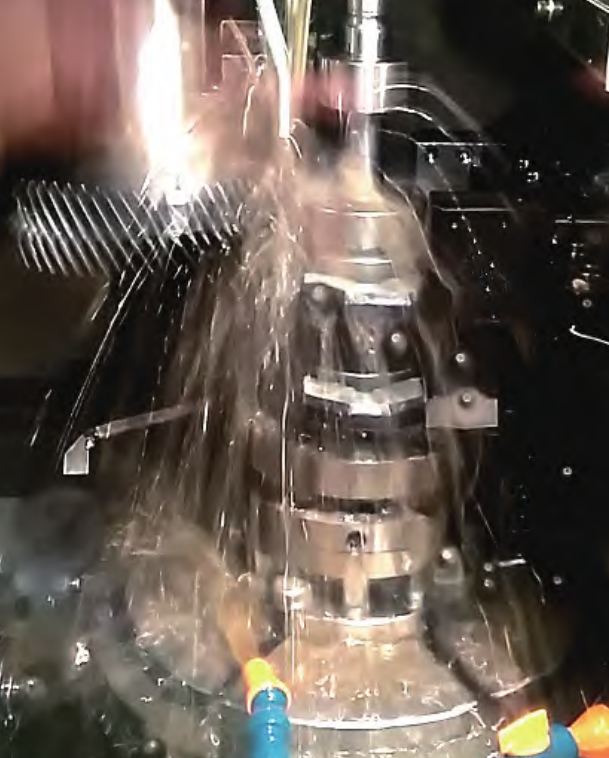
In this experiment, a three-axis MRMG experimental prototype is developed according to the parameters in Table 1. The dynamic loading experimental device of MRMG consists of a driving motor, an input speed and torque sensor 1, an experimental prototype, an output speed and torque sensor 2, three permanent magnet synchronous generators, and three sets of Y-type symmetrical load resistors. The driving motor provides the input speed for the central shaft of the inner permanent magnet ring. The three generators are used as the output end and are connected to each eccentric shaft by a coupling to output voltage in a power splitting manner. The three-phase stator windings of each generator are connected to a set of Y-type symmetrical load resistors to consume the generated power and provide load torque for the eccentric shaft. By changing the input speed of the driving motor while keeping the resistance value constant, different operating conditions of MRMG at different speeds and torques can be obtained. By analyzing the changes of and during stable operation, the characteristics of power splitting, high torque density, and constant transmission ratio of MRMG can be evaluated. In addition, by comparing the power losses and operating efficiencies of MRMG in different transmission modes, the redundancy ability of MRMG in actual operation can be analyzed to verify the effectiveness of the theoretical model established in this paper in the whole working condition dynamic process of MRMG.
5.2 Verification of Steady-State Operating and
In different transmission modes of MRMG, different numbers of loaded eccentric shafts can generate different values under the same speed and torque conditions, resulting in different torque consumptions and values. Therefore, by comparing the and η of different modes in the next section to verify the correctness of equations , it can be proved that the of different modes is also valid. To analyze the changes of and of MRMG at different speeds and torques in the same transmission mode, this paper studies the and of MRMG in the “single input/multiple output” mode when the loads of each eccentric shaft are the same.
Table 2 shows the dynamic loading experiment, theoretical calculation, and simulation data of MRMG in the “single input/multiple output” mode when the loads of each eccentric shaft are the same. The experimental data in the table are obtained from the dynamic loading experimental platform shown. The theoretical calculation data are obtained from the dynamic model shown . The finite element simulation is obtained from the structural model shown in Figure 1 in the Maxwell simulation environment. The and of the experiment, theory, and simulation in Table 2 are calculated by substituting their respective , and into equation (5).
| Inner Permanent Magnet Ring | Outer Permanent Magnet Ring | Eccentric Shaft Total Output Torque /(N·m) | Transmission Ratio | Torque Ratio | ||
|---|---|---|---|---|---|---|
| Input Speed | Input Torque /(N·m) | Output Speed | ||||
| Experiment | -27.70 | -36.11 | 1.10 | -21.75 | -25.18 | |
| Theory | 1.66 | -26.92 | -36.51 | -21.99 | -24.47 | |
| Simulation | -25.98 | -36.01 | -21.69 | -23.62 | ||
| Experiment | -37.28 | -53.64 | 22.07 | -24.53 | ||
| Theory | 2.43 | -36.45 | -53.64 | 1.52 | -22.07 | -23.98 |
| Simulation | -33.84 | -53.17 | 21.88 | -22.26 | ||
| Experiment | 4.04 | -56.29 | -89.81 | 22.23 | -23.95 | |
| Theory | -55.33 | -88.92 | 2.35 | -22.01 | -23.54 | |
| Simulation | -53.82 | -90.17 | -22.32 | -22.90 | ||
| Experiment | 5.06 | -67.22 | -111.81 | 22.10 | -23.84 | |
| Theory | -66.06 | -111.27 | 2.82 | 21.99 | -23.43 | |
| Simulation | -64.79 | 109.35 | -21.61 | -22.98 | ||
| Experiment | 6.07 | 77.46 | -133.86 | 22.05 | -23.76 | |
| Theory | -76.10 | -133.47 | 3.26 | -21.99 | -23.34 | |
| Simulation | -74.45 | -132.09 | -21.76 | -22.84 |
It can be seen from Table 2 and Figure 9 that the curves of and are basically straight lines with a constant slope, and and both increase with the increase of (basically in a linear positive correlation). The average transmission ratio obtained from equation in the dynamic model shown in Figure 2, the measured dynamic data in Figure 8 is -22.04, and the finite element simulation is -21.85. The relative errors of the three are less than 1%, meeting the design requirement of the theoretical transmission ratio . The average torque ratio obtained from equation in the dynamic model shown, the measured dynamic data in Figure 8 is -24.25, and the finite element simulation is -22.91. The relative errors of the three are less than 6%.
5.3 Verification of Transmission Loss
Table 3 shows the relationship data between , , and η of MRMG measured in the dynamic experiment in two modes.
| Inner Permanent Magnet Ring | Outer Permanent Magnet Ring | Shaft 1 (N·m) | Shaft 2/3 | MRMG | ||||
|---|---|---|---|---|---|---|---|---|
| Single Input/Multiple Output Mode with the Same Load on Each Eccentric Shaft | (r/min) | /(N·m) | (r/min) | (N·m) | (W) | η(%) | ||
| 1.66 | -27.70 | -36.11 | 0.37 | 0.61 | 87.17 | |||
| 2.43 | -37.28 | -53.64 | 0.51 | 0.89 | 90.59 | |||
| 4.04 | -56.29 | -89.80 | 0.78 | 1.81 | 92.40 | |||
| 5.06 | -67.22 | -111.81 | 0.94 | 2.60 | 92.70 | |||
| 6.07 | -77.46 | -133.86 | 1.08 | 3.82 | 92.24 | |||
| Single Input/Multiple Output Mode with Different Loads on Each Eccentric Shaft | 1.59 | -18.12 | -34.74 | 0.25 | 0.18 | 0.79 | 73.55 | |
| 2.53 | -23.15 | -54.93 | 0.33 | 0.24 | 1.47 | 75.97 | ||
| 3.92 | -30.87 | -86.34 | 0.46 | 0.34 | 2.36 | 81.34 | ||
| 4.94 | -36.35 | -108.30 | 0.55 | 0.40 | 3.49 | 81.42 | ||
| 6.06 | -42.30 | -133.42 | 0.65 | 0.48 | 4.35 | 83.80 | ||
| Single Input/Single Output Mode | 1.46 | -13.14 | -31.62 | 0.33 | 0.92 | 54.39 | ||
| 2.50 | -19.09 | -54.80 | 0.51 | 2.07 | 58.56 | |||
| 4.09 | -26.57 | -90.07 | 0.78 | 0.00 | 4.02 | 64.65 | ||
| -30.28 | -108.63 | 0.91 | 5.28 | 66.22 | ||||
| 6.06 | -34.14 | -132.07 | 1.07 | 6.87 | 68.30 |
It can be seen from Table that η increases with the increase of and . This is because when the resistance value is constant, the back electromotive force and output current of the permanent magnet synchronous generator are linearly related to , so the provided by the resistance is also proportional to , resulting in increasing with the increase of . According to equations, compared with the increase rate of , the increase rates of and with are relatively small, resulting in an upward trend of η with the increase of and .