
The contact ratio is a fundamental parameter in gear transmission design, directly influencing the smoothness of operation, load distribution, and acoustic behavior. For conventional rigid gear systems, well-established methods exist for its calculation, typically defined as the average number of tooth pairs in contact during the meshing cycle. However, the unique operating principle of the harmonic drive gear presents a significant challenge to applying these traditional methodologies. The harmonic drive gear operates based on controlled elastic deformation, not rigid-body kinematics, necessitating a fundamentally different approach to analyzing its meshing characteristics. This work is dedicated to developing and elaborating a universal, kinematics-based computational framework for determining the contact ratio in harmonic drive gears, applicable to a wide variety of tooth profiles.
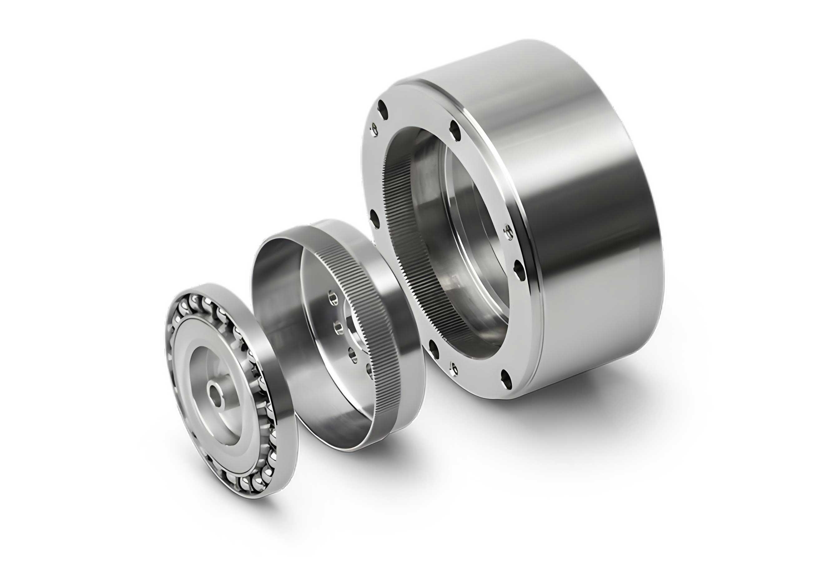
The core innovation of the harmonic drive gear lies in its three key components: a non-deformable circular spline, a flexible spline (or flexspline), and a wave generator. The wave generator, often an elliptical bearing or a cam, is inserted into the flexspline, causing its initially circular rim to deform into an elliptical shape. This deformation brings multiple regions of the flexspline’s teeth into simultaneous engagement with the teeth of the circular spline. As the wave generator rotates, the region of elastic deformation travels with it, creating a progressive, wave-like motion that results in a high reduction ratio between the input (wave generator) and output (flexspline or circular spline). This elastic conjugate motion renders the instantaneous center of rotation for the flexspline tooth non-stationary, a critical distinction from rigid gears.
Due to this inherent difference, the contact ratio for a harmonic drive gear must be redefined in a context that captures its multi-tooth, elastic engagement nature. In this framework, the contact ratio (ε) is defined as the ratio of the total angular zone (across all waves) where a single tooth pair is in mesh to the angular pitch of a single tooth on the circular spline. Mathematically, for a wave generator with N waves, this is expressed as:
$$ \epsilon = \frac{N \cdot \Phi \cdot Z_g}{360} $$
where:
- $\Phi$ is the meshing angular interval for a single tooth pair (in degrees), representing the angle through which the circular spline rotates from the initial to the final contact point of a specific tooth pair.
- $Z_g$ is the number of teeth on the circular spline.
The parameter $\Phi$ is not a fixed geometric property but a dynamic outcome of the interaction between the deformed flexspline and the circular spline. Its determination forms the central computational challenge.
Theoretical Foundation: Willis Theorem and Instantaneous Centers
The proposed method is grounded in the kinematic geometry of planar motion and the fundamental theorem of gear engagement, the Willis theorem. The Willis theorem states that at any point of contact between two conjugate tooth profiles, the common normal to the profiles must pass through the instantaneous center of relative motion (the relative instant center) of the two bodies. This theorem provides the crucial link between the geometry of the teeth and their kinematic state.
To apply this theorem to a harmonic drive gear, we must first understand the motion of the flexspline. The wave generator is considered fixed for analysis (input held stationary). The flexspline undergoes a complex motion comprised of a gross rotation and a superimposed traveling elastic deformation. The instantaneous center of rotation for an individual tooth on the flexspline is not at its geometric center but moves along a specific path relative to the wave generator frame. This path is termed the instantaneous center curve or centrode of the flexspline tooth motion relative to the wave generator.
The relative motion between the flexspline (body 1) and the circular spline (body 2) can be analyzed by finding their relative instantaneous center, $P_{12}$. This point has zero relative velocity between the two bodies at that instant. For two bodies in planar motion, the relative instantaneous center lies on the line connecting their respective absolute instantaneous centers, $O_1$ (for the flexspline tooth) and $O_2$ (for the circular spline, which is simply its geometric center). The location is given by the ratio of their angular velocities. The locus of $P_{12}$ over a cycle of motion is the relative centrode.
Mathematical Derivation of the Contact Interval
1. Wave Generator Profile and Flexspline Deformation
The foundation of the calculation is the shape of the wave generator, which dictates the neutral curve of the deformed flexspline. A common and analytically tractable model is the cosine cam profile. In a polar coordinate system $(ρ_H, ψ)$ attached to the fixed wave generator (frame $σ$), where the polar axis aligns with the major axis of the cam, the radial deflection of the flexspline’s neutral curve is given by:
$$ ρ_H(ψ) = r_c + ω_0 \cos(2ψ) $$
where:
- $r_c$ is the radius of the neutral curve of the undeformed flexspline.
- $ω_0$ is the maximum radial deformation (wave amplitude).
- $ψ$ is the angular coordinate.
The Cartesian coordinates of a point $O_F$ on this curve in the wave generator frame are:
$$ x_{OF} = ρ_H \sin ψ, \quad y_{OF} = ρ_H \cos ψ $$
2. Instantaneous Center of the Flexspline Tooth
Let a coordinate frame $σ^{(F)}$ be rigidly attached to a specific tooth on the flexspline. The instantaneous center of rotation $O_1$ of this tooth, relative to the fixed wave generator frame $σ$, is the point on the tooth that has zero instantaneous velocity. Using kinematics, the coordinates of $O_1$ within the tooth-fixed frame $σ^{(F)}$ are found to be $(0, -ρ)$, where $ρ$ is the radius of curvature of the wave generator cam profile at the contact point $O_F$.
The radius of curvature $ρ$ for a curve defined parametrically by $x(ψ), y(ψ)$ is:
$$ ρ(ψ) = \frac{ \left( \dot{x}_{OF}^2 + \dot{y}_{OF}^2 \right)^{3/2} }{ \dot{x}_{OF} \ddot{y}_{OF} – \ddot{x}_{OF} \dot{y}_{OF} } $$
where dots denote derivatives with respect to $ψ$.
Transforming the coordinates of $O_1$ from the tooth frame $σ^{(F)}$ back to the fixed wave generator frame $σ$ yields its trajectory:
$$
\begin{aligned}
x_{O1}(ψ) &= x_{OF} – ρ(ψ) \sin(ψ + μ(ψ)) \\
y_{O1}(ψ) &= y_{OF} – ρ(ψ) \cos(ψ + μ(ψ))
\end{aligned}
$$
where $μ(ψ)$ is the angular orientation of the flexspline tooth’s symmetric axis relative to the radial line, which is also a function of $ψ$ and can be derived from the cam geometry:
$$ \frac{dμ}{dψ} = \frac{\dot{ρ}_H^2 – \ddot{ρ}_H ρ_H}{ρ_H^2 + \dot{ρ}_H^2} $$
Simulation of these equations reveals that the point $O_1$ traces a star-like closed curve around the cam, a direct consequence of the elliptical deformation.
3. Relative Instantaneous Center between Flexspline and Circular Spline
The circular spline rotates about its fixed geometric center $O_2$ (which coincides with the origin $O$ of frame $σ$). Its absolute instantaneous center is therefore always at $O_2$. The flexspline tooth’s absolute instantaneous center is at $O_1(ψ)$. For two bodies rotating about points $O_2$ and $O_1$ with angular velocities $ω_2$ and $ω_1$ respectively, the relative instantaneous center $P_{12}$ lies on the line $O_2O_1$. Its position is governed by the ratio of angular velocities:
$$ \frac{O_2 P_{12}}{P_{12} O_1} = \frac{ω_1}{ω_2} $$
The angular velocity of the flexspline tooth, $ω_1 = \frac{dθ_F}{dt}$, and of the circular spline, $ω_2 = \frac{dθ}{dt}$, can be related to the cam rotation parameter $ψ$. Their ratio is a key kinematic function. Consequently, the coordinates of the relative instantaneous center $P_{12}$ in the fixed frame $σ$ are:
$$
\begin{aligned}
x_P(ψ) &= \frac{ω_2(ψ)}{ω_2(ψ) – ω_1(ψ)} \cdot x_{O1}(ψ) \\
y_P(ψ) &= \frac{ω_2(ψ)}{ω_2(ψ) – ω_1(ψ)} \cdot y_{O1}(ψ)
\end{aligned}
$$
The locus of $P_{12}$ as $ψ$ varies is the relative centrode for the flexspline and circular spline tooth pair.
4. Determination of Meshing Interval via Willis Theorem
Consider a specific tooth profile on the circular spline. Let its left-side profile be defined in the circular spline’s frame $σ^{(2)}$ by the function $y_R = f(x_R)$. At any potential contact point $M(x_0, y_0)$ on this profile, the equation of the normal line in $σ^{(2)}$ is:
$$ y_R = -\frac{1}{f'(x_0)} (x_R – x_0) + y_0 $$
This line must be transformed into the fixed wave generator frame $σ$ using a rotation matrix defined by the circular spline’s rotation angle $θ$:
$$
\begin{bmatrix} x \\ y \end{bmatrix}_{(σ)} =
\begin{bmatrix} \cos θ & \sin θ \\ -\sin θ & \cos θ \end{bmatrix}
\begin{bmatrix} x_R \\ y_R \end{bmatrix}_{(σ^{(2)})}
$$
Applying this transformation yields the equation of the normal line $n$-$n$ in the fixed frame.
According to Willis theorem, for point $M$ to be an actual contact point at that instant, this normal line $n$-$n$ must pass through the relative instantaneous center $P_{12}$ at the same instant. Therefore, substituting the coordinates $(x_P(ψ), y_P(ψ))$ into the equation of the normal line yields a relation between the cam parameter $ψ$, the tooth profile coordinate $x_0$, and the circular spline rotation angle $θ$.
The meshing interval $Φ$ for one tooth is found by identifying the two limit positions where contact begins and ends. These are typically defined by geometric constraints such as the tip of the circular spline tooth (start of engagement) and the root of the flexspline tooth or another limiting conjugate point (end of engagement). Let these limit points on the circular spline profile be $A(x_A, y_A)$ and $B(x_B, y_B)$. For each limit point:
- Substitute its coordinates $(x_0, y_0)$ into the normal line equation.
- Enforce the Willis condition by substituting the expressions for $x_P(ψ)$ and $y_P(ψ)$ into this line equation.
- Solve the resulting equation to find the corresponding value of the circular spline rotation angle $θ$ (or equivalently, the cam parameter $ψ$ at which this limit contact occurs).
Let the solutions be $θ_A$ and $θ_B$. The single-tooth meshing interval angle $Φ$ is then $|θ_B – θ_A|$. This process is independent of the specific form of $f(x_R)$, making the method universal.
Numerical Example and Computational Procedure
To illustrate the application of this method, we consider a common double-arc (or “S” tooth) profile for the circular spline in a harmonic drive gear. The engagement typically occurs on the convex arc of the circular spline tooth, bounded by the tip circle and the limit point of conjugation. The table below defines the key geometric parameters for the numerical example.
| Parameter | Symbol | Value | Unit |
|---|---|---|---|
| Module | $m$ | 0.5 | mm |
| Number of Waves | $N$ | 2 | – |
| Circular Spline Teeth | $Z_g$ | 152 | – |
| Flexspline Teeth | $Z_f$ | 150 | – |
| Undeformed Flexspline Radius | $r_c$ | $(m \cdot Z_f)/2$ | mm |
| Wave Amplitude | $ω_0$ | Specified by design | mm |
| Circular Spline Pitch Radius | $r_R$ | $(m \cdot Z_g)/2$ | mm |
| Convex Arc Radius | $ρ_α$ | Per tooth standard | mm |
| Profile Angle | $α$ | e.g., 28° | deg |
| Arc Center Offset | $C$ | Per tooth standard | mm |
The left-side convex arc of the circular spline tooth in its own frame $σ^{(2)}$ can be parameterized by an angle $α$ (different from the profile angle, here used as a running parameter):
$$
\begin{aligned}
x_R(α) &= L – ρ_α \cos α + C \\
y_R(α) &= r_R – ρ_α \sin α
\end{aligned}
$$
where $L$ is a datum related to the tooth symmetry line.
The engagement limits are defined by the tip circle radius $r_{ga}$ and the root of the flexspline or the boundary of the working profile. The corresponding limit values $α_{start}$ and $α_{end}$ are determined geometrically. The following computational steps are then executed programmatically (e.g., in C, MATLAB, or Python):
- Define the wave generator profile function $ρ_H(ψ)$ and its derivatives.
- Calculate $x_{O1}(ψ)$, $y_{O1}(ψ)$, and the angular velocity ratio.
- Compute the relative instant center coordinates $x_P(ψ)$, $y_P(ψ)$.
- For the start-of-engagement point (e.g., tooth tip $A$ with $α=α_{start}$):
- Get its coordinates $(x_{R_A}, y_{R_A})$ and the slope of its normal.
- Transform the normal line equation to the fixed frame $σ$, resulting in an equation $F_A(θ, ψ)=0$.
- Substitute $x_P(ψ)$ and $y_P(ψ)$ into $F_A(θ, ψ)=0$ and solve for the pair $(θ, ψ)$ that satisfies it. This yields $θ_A$.
- Repeat step 4 for the end-of-engagement point $B$ (with $α=α_{end}$) to find $θ_B$.
- Calculate $Φ = |θ_B – θ_A|$.
- Compute the contact ratio: $ε = (N \cdot Φ \cdot Z_g) / 360$.
Applying this procedure with the given parameters yields a result that highlights the defining characteristic of the harmonic drive gear. A sample calculation might produce:
| Calculated Parameter | Symbol | Value | Unit |
|---|---|---|---|
| Meshing Interval per Wave per Tooth Pair | $Φ$ | ~53.86 | deg |
| Theoretical Contact Ratio | $ε$ | ~45.5 | – |
This exceptionally high contact ratio, orders of magnitude greater than that of typical spur or helical gears (which are usually between 1 and 2), quantifies the superior load-sharing capability and smoothness of the harmonic drive gear. It confirms that dozens of tooth pairs are in contact simultaneously across the circumference.
Discussion on Generality and Practical Considerations
The derived method possesses significant generality. The process for finding the relative instant center $P_{12}$ depends solely on the wave generator profile $ρ_H(ψ)$ and the resulting flexspline deformation kinematics. It is completely independent of the specific tooth profile geometry defined by $f(x_R)$. Therefore, this same computational framework can be applied to analyze the contact ratio of harmonic drive gears with involute, double-arc, triangular, or any novel proprietary tooth profile. This makes it an invaluable tool for evaluating and comparing the meshing performance of new harmonic drive gear tooth designs.
It is crucial to distinguish between the theoretical contact ratio calculated above and the effective contact ratio under operational conditions. The theoretical calculation assumes perfect geometry, zero load, and ideal conjugate action. In a real harmonic drive gear, several factors influence the actual number of load-bearing tooth pairs:
- Load-Induced Deflections: Under torque, the flexspline, wave generator bearing, and teeth themselves experience additional elastic deformations. This can slightly shift the actual contact points and pressure distribution from their theoretical positions, potentially altering the effective engagement zone.
- Manufacturing Tolerances and Errors: Deviations in tooth profile, wave generator geometry, and assembly misalignments will affect the conjugate conditions and load sharing.
- Tooth Surface Modification: Intentional profile modifications (tip and root relief, lead crowning) are often applied to improve stress distribution and accommodate misalignment. These modifications technically reduce the strictly conjugate zone but enhance performance, requiring the contact ratio calculation to consider the “functional” profile.
Thus, the theoretical contact ratio serves as a powerful upper-bound benchmark and a comparative index. For precise design, finite element analysis (FEA) considering elastic deformations under load is often employed to determine the actual load distribution factor, which is closely related to the effective contact ratio.
The high contact ratio is the root cause of several key advantages of the harmonic drive gear:
- High Torque Capacity and Load Distribution: The load is distributed over many teeth, drastically reducing the stress on individual tooth pairs compared to conventional gears with similar size.
- Exceptional Torsional Stiffness and Precision: The large number of engaged teeth provides high resistance to angular deflection under load, contributing to precise positioning.
- Smooth and Quiet Operation: The continuous, multi-tooth engagement minimizes torque ripple and vibration, leading to low acoustic noise.
Conclusion
This work has presented a comprehensive, kinematics-based methodology for calculating the contact ratio in harmonic drive gears. By redefining the contact ratio in terms of the meshing angular interval and leveraging the fundamental Willis theorem combined with the analysis of instantaneous centers of motion, a universal computational framework is established. The derivation demonstrates that the path of the relative instant center is a function purely of the wave generator’s kinematics, while the application of the Willis theorem ties this kinematics to the specific tooth profile geometry to determine the engagement boundaries.
The resulting formula, $ε = (N \cdot Φ \cdot Z_g)/360$, when populated via the described procedure, quantitatively reveals the extraordinary multi-tooth engagement characteristic of the harmonic drive gear, with contact ratios typically exceeding 30 and often reaching 50 or more. This high value is the fundamental kinematic explanation for the transmission’s renowned high torque density, stiffness, and smooth operation.
This method’s independence from tooth profile specifics renders it a potent analytical tool for researchers and engineers developing new tooth forms for harmonic drive gears. It provides a standardized metric—the theoretical contact ratio—to assess and compare the inherent meshing quality and potential load-sharing capability of novel designs before proceeding to more complex and costly loaded-tooth contact analysis or prototype testing. Future work may focus on integrating this kinematic model with elastostatic finite element models to bridge the gap between theoretical and effective load-bearing contact ratio under operational conditions.