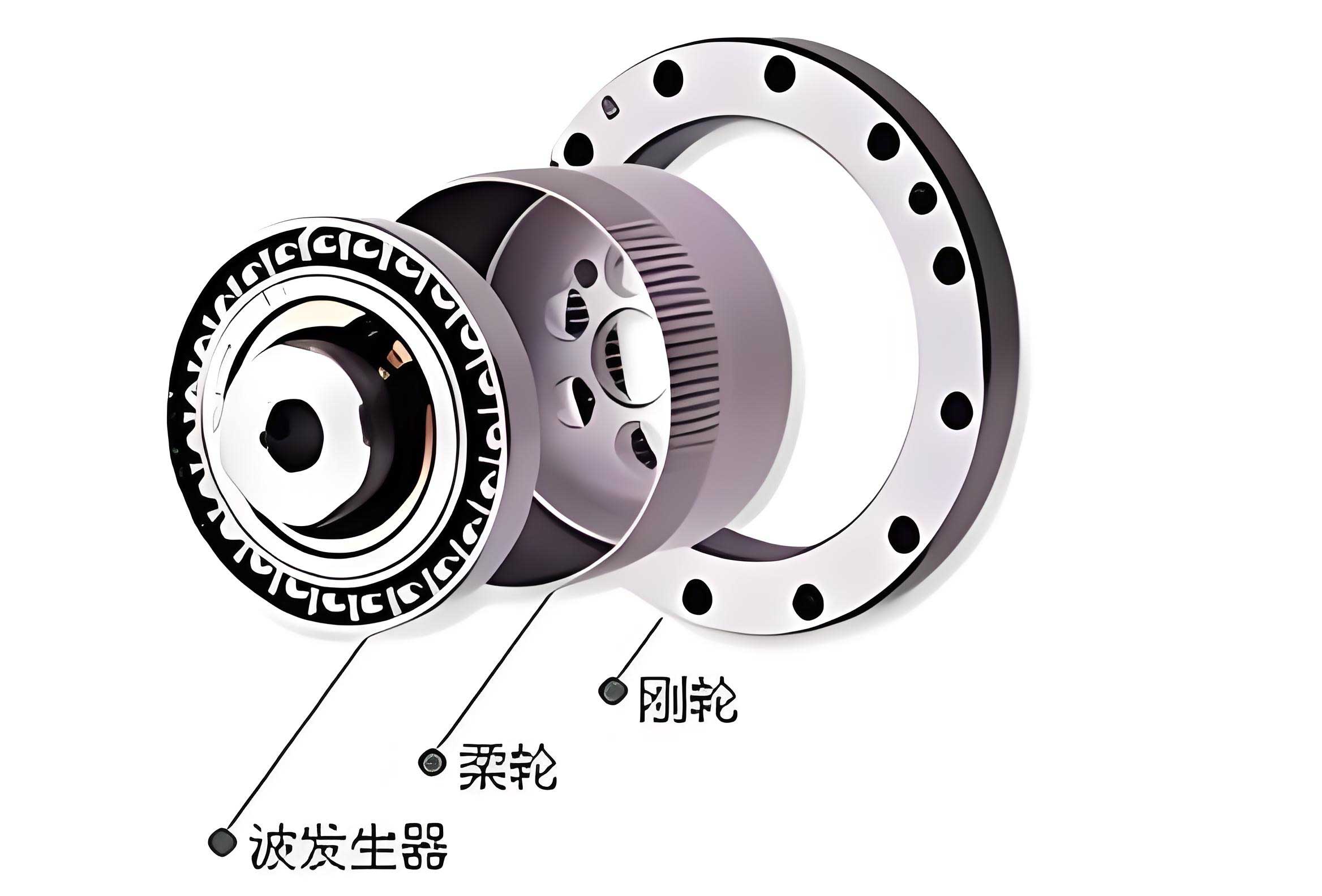
Conjugate Tooth Profile Generation for Strain Wave Gears

The pursuit of high-precision, compact, and high-torque transmission systems has consistently driven innovation in gear technology. Among these, the strain wave gear, also known as harmonic drive, stands out due to its exceptional features: high reduction ratios in a single stage, zero-backlash operation, compact size, and high positional accuracy. These attributes make it indispensable in robotics, aerospace, satellite positioning systems, and high-end industrial automation. At the heart of a strain wave gear’s performance lies the precise meshing between its three primary components: the rigid circular spline, the flexible spline (or flexspline), and the wave generator. The core challenge in designing high-performance strain wave gear lies in determining the exact conjugate tooth profile for the rigid spline that ensures smooth, continuous, and interference-free contact with the flexspline’s teeth throughout the engagement cycle. This task is fundamentally governed by the complex, elastic deformation of the flexspline induced by the wave generator.

Traditional theoretical methods for solving conjugate profiles rely on an idealized deformation function derived from elastic shell theory, assuming the flexspline’s neutral line does not elongate and its generators remain straight. However, this simplification often diverges from the real mechanical state of the assembly, particularly when considering factors like the influence of the teeth themselves, axial constraints, and the non-uniform deformation along the flexspline’s length. These discrepancies can lead to suboptimal meshing conditions, manifested as non-uniform backlash, localized stress concentrations, premature wear, and even tooth interference, ultimately compromising the transmission’s efficiency, lifespan, and precision.

This article presents a comprehensive methodology for generating the conjugate tooth profile of a rigid spline in a strain wave gear. The approach synergistically combines finite element analysis (FEA), advanced curve fitting techniques, and kinematic simulation based on the envelope theory. The primary innovation lies in replacing the classical theoretical deformation function with a high-fidelity, empirically derived function extracted from a detailed finite element model of the flexspline’s initial assembly state. This method accounts for the actual geometric and boundary conditions, providing a more accurate foundation for the subsequent kinematic and meshing analysis.

Theoretical Foundation of Meshing in Strain Wave Gears

The kinematic model for solving the conjugate profile is established based on the principle of envelope generation. We consider a configuration where the rigid spline is fixed, the wave generator is the input, and the flexspline is the output. Three coordinate systems are defined, as illustrated in Figure 1 of the source material.

Global Coordinate System $ C_G(x_G, y_G) $: Fixed to the rigid spline. Its origin $ O_G $ coincides with the transmission’s center of rotation, and its $ y_G $-axis aligns with the symmetry line of a rigid spline tooth space.
Local Coordinate System $ C_R(x_R, y_R) $: Fixed to the flexspline. Its origin $ O_R $ is the intersection of a tooth’s symmetry line and the flexspline’s deformed neutral curve (often called the “prime curve”). Its $ y_R $-axis aligns with the symmetry line of the flexspline tooth profile.
Local Coordinate System $ C_0(x_0, y_0) $: Fixed to the wave generator. Its origin $ O_0 $ coincides with $ O_G $, and its $ y_0 $-axis aligns with the major axis of the elliptical wave generator.

The fundamental task is to find the rigid spline profile $ (x_G(t), y_G(t)) $ that is the envelope of the family of curves generated by the flexspline tooth profile $ (x_R(t), y_R(t)) $ as it moves according to the deformation kinematics. The coordinate transformation from the flexspline system $ C_R $ to the global system $ C_G $ involves both a rotation and a translation that are functions of the wave generator’s rotation angle $ \phi $ and the flexspline’s deformation.

The transformation matrix $ \mathbf{M}_{RG} $ is given by:

$$ \begin{bmatrix} x_G(t) \\ y_G(t) \\ 1 \end{bmatrix} = \mathbf{M}_{RG} \begin{bmatrix} x_R(t) \\ y_R(t) \\ 1 \end{bmatrix} = \begin{bmatrix} \cos\Phi & \sin\Phi & \rho \sin\gamma \\ -\sin\Phi & \cos\Phi & \rho \cos\gamma \\ 0 & 0 & 1 \end{bmatrix} \begin{bmatrix} x_R(t) \\ y_R(t) \\ 1 \end{bmatrix} $$

The meshing condition, which ensures contact between conjugate profiles, is derived from the envelope theory and is expressed by the following equation:

$$ \frac{\partial x_G}{\partial \phi} \frac{\partial y_G}{\partial t} – \frac{\partial y_G}{\partial \phi} \frac{\partial x_G}{\partial t} = 0 $$

Within these equations, the key parameters are defined as follows:

$ \rho $: The polar radius of the deformed neutral curve of the flexspline (prime curve).
$ \Phi $: The angle between the $ y_R $-axis and the $ y_G $-axis when the rigid spline is fixed. It is the sum of the wave generator’s rotation angle $ \phi $ and the flexspline’s rotation $ \gamma $.
$ \gamma $: The rotational displacement of the flexspline, related to the wave generator’s angle by $ \gamma = \frac{U}{z_1} \phi + \frac{\upsilon}{r_m} $, where $ U $ is the wave number (typically 2), $ z_1 $ is the number of flexspline teeth, and $ \upsilon $ is the tangential deformation.
$ \mu $: The inclination angle of the flexspline tooth due to deformation, calculated as $ \mu = \arctan(\rho’ / \rho) \approx \frac{1}{r_m} \frac{d\omega}{d\phi} $, where $ \omega $ is the radial deformation and $ r_m $ is the nominal radius of the flexspline’s neutral surface.

Therefore, the complete expression for $ \Phi $ is:

$$ \Phi = \mu + \gamma = \frac{1}{r_m} \frac{d\omega}{d\phi} + \frac{U}{z_1} \phi + \frac{\upsilon(\phi)}{r_m} $$

The successful application of this theoretical framework hinges on the accurate determination of the radial deformation function $ \omega(\phi) $ and the tangential deformation function $ \upsilon(\phi) $. In classical theory, these are derived as complex elliptical integrals. Our methodology seeks to determine these functions directly from a simulated physical model of the assembled strain wave gear.

Finite Element Analysis for Initial Deformation

To capture the true initial deformation state of the flexspline after the wave generator is inserted (under no-load conditions), a detailed 3D finite element model is constructed. The analysis focuses on a common configuration: a cup-type flexspline with a double-circular-arc tooth profile, a rigid circular spline, and an elliptical cam wave generator.

Model Setup and Assumptions:

Geometry: A full 360-degree model of both the flexspline and a simplified wave generator is used to avoid symmetry assumptions that might mask asymmetric deformation modes. The teeth on the flexspline’s rim are explicitly modeled, as their presence significantly affects the stiffness and deformation pattern of the structure.
Wave Generator Simplification: The wave generator assembly (cam and flex bearing) is modeled as a single rigid ring. Its outer contour is defined as the offset curve of the cam’s elliptical profile by the thickness of the flex bearing, effectively representing the contact surface that pushes against the flexspline’s inner wall.
Materials:
- Flexspline: 35CrMnSiA steel, heat-treated and nitrided. Young’s Modulus $ E = 209 $ GPa, Poisson’s ratio $ \nu = 0.295 $.
- Wave Generator (simplified ring): 45 steel. $ E = 209 $ GPa, $ \nu = 0.269 $.
Mesh: 8-node linear reduced-integration hexahedral elements (C3D8R in Abaqus) with hourglass control are employed for their efficiency in contact analysis.
Constraints and Loading:
1. The wave generator is constrained as a rigid body. Its upper and lower semi-elliptical halves are given prescribed displacements of $ +\omega_0 $ and $ -\omega_0 $ respectively, simulating the insertion process. $ \omega_0 $ is the nominal radial deformation coefficient ($ \omega^* $) multiplied by the module $ m $.
2. The axial displacement of the flexspline’s open end is restricted to simulate the effect of the mounting flange or diaphragm.
3. Surface-to-surface contact is defined between the wave generator’s outer surface (master) and the flexspline’s inner surface (slave), considering finite sliding.

Results and Discussion:

The FEA results reveal deformation patterns that deviate meaningfully from the classical theoretical assumptions.

Radial Deformation ($ \omega $): The maximum radial expansion occurs along the major axis, but its value (e.g., 0.553 mm for a nominal $ \omega_0 = 0.5 $ mm) exceeds the theoretical prediction. Conversely, at the minor axis, the contraction (e.g., -0.557 mm) is also greater than theoretical. This indicates a more severe “ovalization” than idealized theory suggests.
Tangential Deformation ($ \upsilon $): The maximum tangential displacement is found near the regions at approximately ±45° from the major axis at the cup’s open end, with magnitudes (e.g., 0.293 mm) larger than the theoretical value (typically $ \omega_0/2 = 0.25 $ mm).
Key Observations: The analysis clearly shows that the open end of the cup flexspline wraps around the wave generator, a phenomenon not captured by simple plane-strain models. This helps explain the characteristic wear patterns observed on the leading edge of flex bearings in practice. Furthermore, the deformation is not uniform along the axis; the flexspline’s generators tilt, meaning the inner wall does not maintain perfect, full-length contact with the wave generator, contradicting a common theoretical simplification.

The data of primary interest for conjugate profile generation is the deformation of the neutral surface of the rim’s middle cross-section. The radial ($ \omega_i $) and tangential ($ \upsilon_i $) displacements of nodes on this neutral contour, sampled at discrete angular positions $ \phi_i $, are extracted from the FEA results. This discrete dataset $ \{ \phi_i, \omega_i, \upsilon_i \} $ forms the empirical basis for defining the deformation functions, replacing the classical theoretical formulas.

Table 1: FEA Model Key Parameters
Parameter	Symbol	Value
Module	$ m $	0.5 mm
Flexspline Teeth	$ z_1 $	200
Rigid Spline Teeth	$ z_2 $	202
Radial Deformation Coefficient	$ \omega^* $	1.0
Nominal Radial Deformation	$ \omega_0 = \omega^* m $	0.5 mm
Rim Wall Thickness	$ \delta $	0.9 mm

Deriving Deformation Functions via Curve Fitting

The discrete FEA data must be converted into continuous mathematical functions $ \omega(\phi) $ and $ \upsilon(\phi) $ to be used in the kinematic equations. Given the periodic and integrable nature of the deformation in a strain wave gear, a Fourier series representation is a natural choice. For practicality and excellent convergence, a sum of sine functions is selected as the fitting model.

The general form of the fitting function is:

$$ f(\phi) = \sum_{i=1}^{n} a_i \sin(b_i \phi + c_i) $$

where $ a_i, b_i, c_i $ are the amplitude, frequency, and phase coefficients for the $ i $-th term, and $ n $ is the number of terms. The optimal value of $ n $ and the corresponding coefficients are determined by minimizing the error between the fitting function and the FEA data points. The quality of the fit is assessed using standard statistical metrics:

Sum of Squares Due to Error (SSE): Measures the total deviation of the fit from the data. Closer to 0 is better.
Root Mean Square Error (RMSE): The standard error of the fit. Closer to 0 is better.
R-square (R²) and Adjusted R-square: Measures how successful the fit is in explaining the variation of the data. Values closer to 1 indicate a better fit.

Using a curve fitting toolbox (like the one in MATLAB), various fits with different numbers of terms $ n $ are evaluated. A model with $ n=3 $ sine terms often provides an excellent balance between accuracy and complexity for strain wave gear deformation.

Table 2: Optimal Fit Coefficients for Radial Deformation $ \omega(\phi) $
Coefficient Set	Value
$ a_1, a_2, a_3 $	[0.5272, 0.02677, 0.007596] mm
$ b_1, b_2, b_3 $	[1.987, 5.965, 4.033] rad⁻¹
$ c_1, c_2, c_3 $	[1.611, 1.694, -9.533] rad
SSE	3.233e-3 mm²
RMSE	4.69e-3 mm
Max Fitting Error	0.00107 mm (~1/517 of max ω)

The extremely small RMSE and maximum fitting error (only 0.00107 mm, which is negligible compared to the deformation magnitude) confirm the high fidelity of the fitted function $ \omega(\phi) $. When plotted against the classical theoretical deformation function, the fitted curve reveals a consistent deviation, with a maximum difference of about 0.053 mm, underscoring the importance of using FEA-derived data.

Table 3: Optimal Fit Coefficients for Tangential Deformation $ \upsilon(\phi) $
Coefficient Set	Value
$ a_1, a_2, a_3 $	[0.2956, 0.01807, 0.01897] mm
$ b_1, b_2, b_3 $	[2.013, 0.2032, 4.067] rad⁻¹
$ c_1, c_2, c_3 $	[3.090, -1.919, -1.909] rad
SSE	4.515e-3 mm²
RMSE	7.044e-3 mm
Max Fitting Error	0.00053 mm (~1/553 of max υ)

Similarly, the tangential deformation function $ \upsilon(\phi) $ is fitted with high precision (max error ~0.00053 mm). These two fitted functions, $ \omega(\phi) $ and $ \upsilon(\phi) $, now serve as the accurate, empirically based kinematic input for the conjugate profile generation of the strain wave gear, replacing the less precise theoretical formulas.

Kinematic Simulation and Envelope Generation

With the deformation functions defined, the process of generating the conjugate rigid spline profile proceeds through kinematic simulation and mathematical enveloping. The procedure is implemented computationally, for example, in MATLAB or a similar environment.

Step 1: Define the Flexspline Tooth Profile.
The known flexspline profile, often a double-circular-arc or an involute, is defined in its local coordinate system $ C_R $ as a set of discrete points $ \mathbf{P}_R(t) = [x_R(t), y_R(t)]^T $, where $ t $ is a parameter defining the curve.

Step 2: Simulate the Motion.
For a full engagement cycle of a single tooth, the wave generator rotation angle $ \phi $ is varied incrementally from 0 to $ 2\pi $. For each discrete angle $ \phi_k $:

Calculate the current deformation values $ \omega(\phi_k) $ and $ \upsilon(\phi_k) $.
Calculate the associated angles $ \mu(\phi_k) $, $ \gamma(\phi_k) $, and finally $ \Phi(\phi_k) = \mu(\phi_k) + \gamma(\phi_k) $.
Calculate the polar radius of the prime curve: $ \rho(\phi_k) = r_m + \omega(\phi_k) $.
Construct the transformation matrix $ \mathbf{M}_{RG}(\phi_k) $ using $ \Phi(\phi_k) $, $ \rho(\phi_k) $, and $ \gamma(\phi_k) $.
Transform all points of the flexspline tooth profile from $ C_R $ to the global system $ C_G $:
$$ \mathbf{P}_G(t, \phi_k) = \mathbf{M}_{RG}(\phi_k) \cdot \mathbf{P}_R(t) $$
This yields the position of the flexspline tooth at instant $ \phi_k $.

Step 3: Generate the Envelope.
The collection of all transformed curves $ \mathbf{P}_G(t, \phi_k) $ for all $ \phi_k $ forms a family of curves. The envelope of this family is the set of points where consecutive curves are infinitesimally close, satisfying the meshing condition derived earlier. Numerically, this envelope can be found by solving the meshing equation for each point on the flexspline profile across the range of $ \phi $, or by using specialized algorithms that detect the boundary curve of the swept volume. The resulting set of points $ \mathbf{Q}_j = [x_{G_j}, y_{G_j}]^T $ represents the theoretical conjugate profile of the rigid spline for the strain wave gear.

Step 4: Practical Profile Fitting.
The mathematically generated envelope $ \{ \mathbf{Q}_j \} $ may contain points outside the practical working zone or may not conform to a standard manufacturable profile. Therefore, a practical rigid spline profile is obtained by fitting a suitable curve to the relevant portion of the envelope points. A common and effective choice for double-circular-arc systems is a circular arc – straight line – circular arc composite curve. The parameters of these arcs and line are optimized using a least-squares fitting algorithm to minimize the deviation from the theoretical envelope points $ \mathbf{Q}_j $.

The fitting error is rigorously checked. For instance, the maximum deviation between the fitted circular-arc profile and the theoretical envelope points might be on the order of nanometers (e.g., 0.00869 μm), which is orders of magnitude smaller than the allowable form error for high-precision gears. This confirms that from an engineering standpoint, the fitted profile is an excellent and manufacturable representation of the true conjugate profile for the strain wave gear.

Table 4: Summary of the Proposed Methodology
Step	Tool/Action	Output	Purpose
1. Physical Simulation	Finite Element Analysis (Abaqus)	Discrete deformation data $ \omega_i, \upsilon_i $	Capture real assembly deformation, accounting for teeth and boundary conditions.
2. Function Derivation	Curve Fitting (e.g., MATLAB)	Continuous functions $ \omega(\phi), \upsilon(\phi) $	Create accurate, simple kinematic input from FEA data.
3. Kinematic Modeling	Coordinate Transformation & Motion Simulation	Family of flexspline tooth positions $ \mathbf{P}_G(t, \phi) $	Simulate the path of the flexspline tooth relative to the fixed rigid spline.
4. Conjugate Solution	Envelope Theory / Numerical Detection	Set of conjugate profile points $ \{ \mathbf{Q}_j \} $	Find the theoretical rigid spline profile that maintains continuous contact.
5. Engineering Design	Least-Squares Curve Fitting	Manufacturable profile (e.g., circular arcs)	Generate a practical, high-precision tooth profile for the rigid spline.

Discussion and Conclusion

This article has detailed a robust and practical methodology for solving the conjugate tooth profile in a strain wave gear drive. The core innovation is the integration of finite element analysis into the traditional envelope theory framework. By using FEA to determine the initial deformation functions $ \omega(\phi) $ and $ \upsilon(\phi) $, the method effectively bridges the gap between idealized analytical models and the complex physical reality of the assembled strain wave gear components.

The key advantages of this approach are:

Increased Accuracy: The FEA-derived deformation functions account for the influence of the teeth, the cup geometry, and realistic boundary conditions, leading to a more accurate representation of the flexspline’s kinematic state than classical theory.
Practicality: The use of curve fitting yields simple, explicit mathematical functions that are easily incorporated into kinematic simulation and envelope-solving algorithms.
Validation Path: The method is inherently verifiable. The FEA model can be correlated with strain gauge measurements on a physical prototype, and the final conjugate profile’s performance can be analyzed through loaded tooth contact analysis (LTCA) using the same FEA tools, creating a closed-loop design process.

The successful generation of a rigid spline profile via this method, with fitting errors in the nanometer range compared to the theoretical envelope, demonstrates its viability. It provides a powerful reference for the design and optimization of high-performance strain wave gear transmissions. Future work naturally extends from this foundation:

Loaded Deformation Analysis: The initial deformation (no-load) functions can be augmented or replaced by functions derived from FEA under full operational torque. This would enable the design of profile modifications that optimize load distribution and minimize stress under working conditions.
Dynamic Simulation: The kinematic model can be extended to include dynamic effects, such as tooth separation under high acceleration or impact loads, to design profiles for highly dynamic applications.
Multi-objective Optimization: The entire process—from FEA parameters to final profile fitting—can be embedded within an optimization loop to simultaneously minimize stress, maximize efficiency, ensure uniform backlash, and reduce wear.

In conclusion, the conjugate profile generation for strain wave gears is a critical design task that directly impacts the transmission’s core performance metrics. The methodology combining finite element analysis, empirical curve fitting, and kinematic envelope simulation offers a significant advancement over purely theoretical approaches. It provides engineers with a more reliable and accurate toolset for designing the precise, high-performance conjugate tooth profiles that enable the exceptional capabilities of modern strain wave gear drives.