
In the field of modern gear design and manufacturing, particularly for complex geometries like hypoid gears, achieving an accurate digital representation of the tooth flank is paramount. Traditional analytical descriptions can be limiting for free-form or precisely machined surfaces. This is where the power of Non-Uniform Rational B-Spline (NURBS) surfaces becomes indispensable. From a practical engineering standpoint, I have found that utilizing NURBS for the reverse engineering or mathematical modeling of hypoid gear tooth flanks offers unparalleled flexibility and precision. This article details my approach and analysis on fitting these critical surfaces, focusing on the factors that govern accuracy and the methodologies for efficient error evaluation.
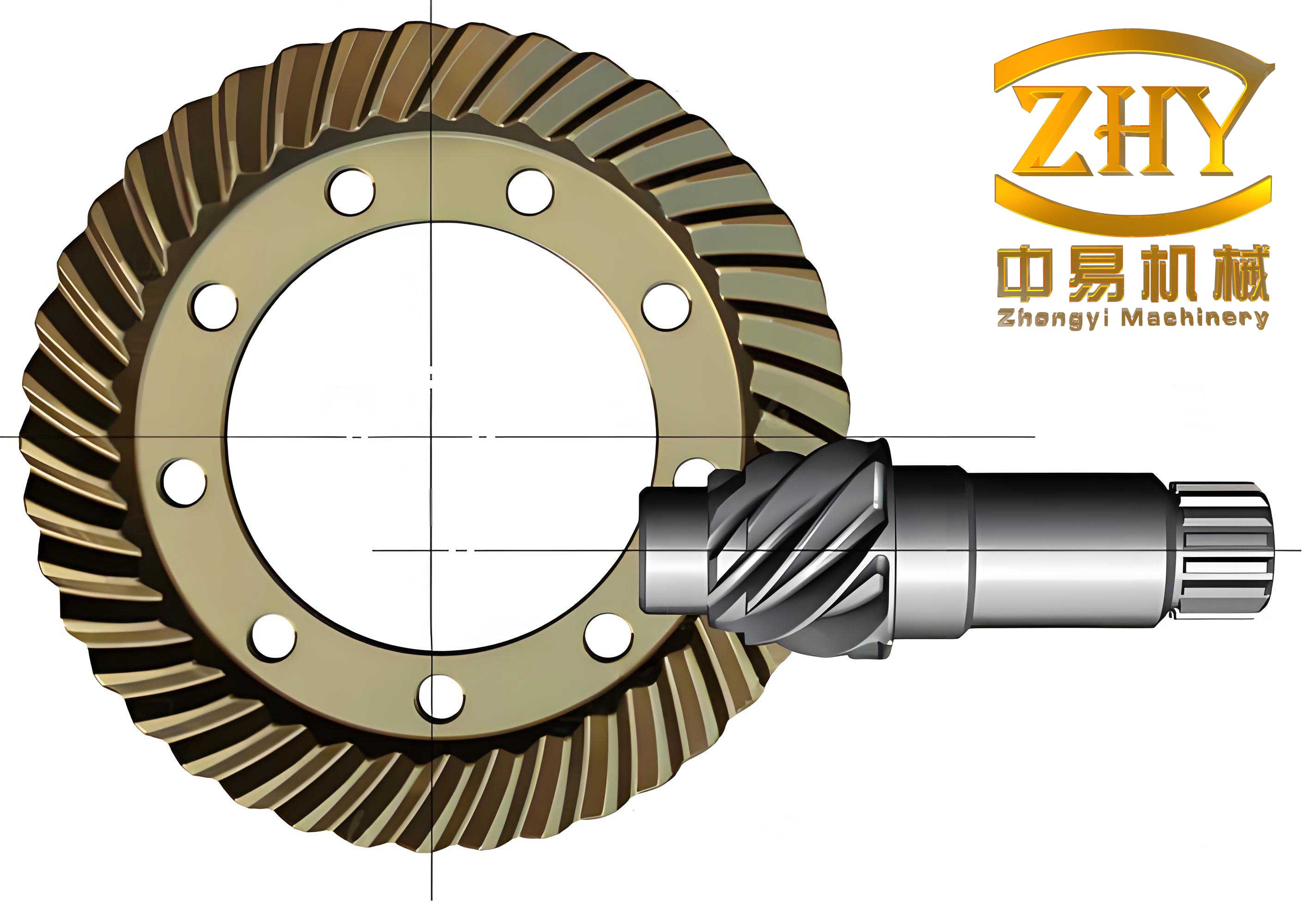
The geometry of hypoid gears is intrinsically complex, featuring skewed axes and a combination of rolling and sliding motions. This results in tooth flanks that are highly curvaceous and non-developable. Obtaining a high-fidelity computer model is essential for advanced analyses such as contact simulation, stress calculation, transmission error prediction, and direct integration into CAD/CAM systems for manufacturing. While the theoretical generation of hypoid gear surfaces can be derived from machine-tool settings and kinematic relations, a complementary and powerful method involves fitting a NURBS surface to a dense point cloud obtained from either simulated machining or physical coordinate measurement machines (CMM). This process, essentially a sophisticated form of reverse engineering, aims to encapsulate the true geometry within a versatile mathematical formulation.
Mathematical Foundation of NURBS Surface Fitting
The core of this methodology lies in the NURBS representation. A NURBS surface of degree k-1 in the u direction and degree l-1 in the v direction is defined by a bidirectional control net, weight factors, and knot vectors. Its rational form is given by:
$$S(u, v) = \frac{\sum_{i=0}^{n} \sum_{j=0}^{m} N_{i,k}(u) N_{j,l}(v) w_{i,j} P_{i,j}}{\sum_{i=0}^{n} \sum_{j=0}^{m} N_{i,k}(u) N_{j,l}(v) w_{i,j}}$$
where:
- $P_{i,j}$ are the control points forming a bidirectional net.
- $w_{i,j}$ are the corresponding positive weight factors.
- $N_{i,k}(u)$ and $N_{j,l}(v)$ are the non-uniform B-spline basis functions of degree k-1 and l-1, defined on knot vectors $U$ and $V$ respectively.
The process of fitting such a surface to known data points, often called surface interpolation or approximation, involves determining the unknown control points $P_{i,j}$ and weights $w_{i,j}$ from a set of data points $Q_{r,s}$ (also called 型值点) which lie on the target surface—in this case, the hypoid gear tooth flank. A highly effective strategy leverages the projective transformation and homogeneous coordinates. By converting the 3D data points and their associated weights into 4D homogeneous space, the rational NURBS fitting problem is transformed into a non-rational B-spline fitting problem, which is linear in its unknowns. The steps are as follows:
- For each 3D data point $Q_{r,s}$ with an implied or assigned weight $\omega_{r,s}$, define its 4D homogeneous coordinate: $Q_{r,s}^* = (\omega_{r,s} \cdot Q_{r,s},\ \omega_{r,s})$.
- Perform a standard bi-directional B-spline interpolation/approximation in 4D space on the points $Q_{r,s}^*$ to solve for the 4D control points $P_{i,j}^*$.
- Revert the solved 4D control points back to 3D Euclidean space and their weights:
$$P_{i,j} = \frac{\text{First three components of } P_{i,j}^*}{\text{Fourth component of } P_{i,j}^*}, \quad w_{i,j} = \text{Fourth component of } P_{i,j}^*$$
This method simplifies the computational complexity significantly. The accuracy of the final fitted NURBS surface for the hypoid gear tooth flank is not automatic; it is profoundly influenced by several interdependent factors during the fitting process.
Critical Factors Influencing Fitting Accuracy for Hypoid Gears
When reconstructing the intricate surface of hypoid gears, meticulous attention must be paid to the following parameters:
1. Selection and Distribution of Data Points: The foundational input is a cloud of points sampled from the true hypoid gear tooth surface. The rule here is that the density of these data points should be non-uniform and should reflect the local curvature. Areas of high curvature, such as the fillet region or the topographical extremes on a highly curved pinion flank, require a denser sampling. Conversely, relatively flatter regions can be described with fewer points. For hypoid gears, the driven gear (often the larger wheel) machined by a Formate or face-milling process may have a simpler curvature along the profile direction, allowing for sparser sampling in that parameter. The pinion, however, with its complex longitudinally crowned and profile-modified surface, demands a dense and well-distributed grid in both parametric directions ($u$ and $v$). A trade-off exists: more points increase potential accuracy but also increase computational load and can lead to numerical instability or an overly “wiggly” surface. The goal is to use the minimum number of points that capture the essential shape of the hypoid gear tooth within a specified tolerance.
2. Parameterization and Knot Vector Calculation: Assigning a $(u, v)$ parameter value to each data point is a crucial step known as parameterization. A poor parameterization distorts the surface mapping, leading to fitting errors. The most common and robust method for free-form shapes is the cumulative chord length method. For a sequence of data points $Q_0, Q_1, …, Q_s$, the parameter for the $t$-th point is calculated as:
$$u_t = \frac{\sum_{i=0}^{t-1} ||Q_{i+1} – Q_i||}{\sum_{i=0}^{s-1} ||Q_{i+1} – Q_i||}, \quad \text{with } u_0 = 0$$
This method reflects the geometric spacing of the points, which is vital for the subsequent non-uniform knot vector generation. The knot vectors $U$ and $V$ are then determined from these parameters, typically using the averaging technique to ensure a well-conditioned system matrix. The non-uniformity of the knot vectors, directly derived from this chord-length parameterization, is what allows NURBS to adaptively fit the irregularly spaced data points from a hypoid gear scan much more effectively than uniform methods.
3. Determination of Boundary Conditions: The surface fitting process is usually decomposed into a series of curve fittings along one parameter direction, then the other. In each curve fit, the number of unknown control points exceeds the number of data point equations. The missing equations come from boundary conditions. For open curves/surfaces like a gear tooth flank, the natural choice is often the specification of end tangents (first derivatives). The accuracy of these specified tangent vectors, particularly their magnitudes, is critical. An incorrect magnitude, even with the correct direction, will cause the fitted curve (and consequently the surface) to oscillate near the boundary, creating a “ripple” effect that propagates inward. For hypoid gears, where the tooth edges are often contact boundaries, such inaccuracies are unacceptable. The most consistent method is to derive the end tangent vectors based on the same chord-length parameterization used for the knot sequence. The derivative of the curve with respect to this arc-length-like parameter provides a geometrically meaningful and stable boundary condition, minimizing unwanted oscillations in the fitted hypoid gear surface.
4. Error Evaluation and the Optimization Loop: After fitting, the quality must be quantified. The fitting error at a given validation point $M (X, Y, Z)$—a point on the real hypoid gear not used in the data set—is defined as the shortest distance from $M$ to the fitted NURBS surface $S(u,v)$. Computing this directly requires finding the parameters $(u_0, v_0)$ that minimize the distance, which is a non-linear optimization problem. A fast and effective approach is to set up an unconstrained optimization model:
$$\text{Minimize } f(u, v) = [S_x(u,v) – X]^2 + [S_y(u,v) – Y]^2$$
$$\text{for } u, v \in [0, 1]$$
Here, $S_x$ and $S_y$ are the X and Y components of the surface point. For a hypoid gear, if the projection of the tooth flank in the XY-plane is monotonic, this method is efficient. Algorithms like the steepest descent or conjugate gradient methods can quickly find $(u_0, v_0)$. Once found, the primary error can be assessed as the deviation in Z-direction $\Delta Z = |S_z(u_0,v_0) – Z|$, or more rigorously as the Euclidean distance $\Delta r = ||S(u_0,v_0) – M||$. The maximum of $\Delta r$ over a set of validation points represents the global fitting error of the NURBS model for that hypoid gear tooth.
Application to Hypoid Gear Tooth Flank Fitting: A Detailed Workflow
Applying the above principles to hypoid gears involves a structured workflow. Let’s consider fitting the convex side of a hypoid pinion, which is typically more complex than the gear.
- Data Acquisition: Obtain a high-density point cloud from the pinion tooth flank, either via CMM measurement or high-fidelity simulation of the manufacturing process (e.g., face-hobbing or face-milling simulation).
- Data Preprocessing & Selection: Organize the points into a roughly grid-like topology (e.g., points along successive profile lines). From this dense cloud, strategically select a subset to serve as the primary data points for fitting. As discussed, select more points in regions of high curvature (toe, heel, tip, root) and fewer in flatter regions. The following table suggests a strategy:
| Region on Hypoid Pinion | Curvature Characteristic | Recommended Data Point Density |
|---|---|---|
| Toe and Heel (ends of lengthwise curve) | High | High |
| Tip and Root (ends of profile curve) | High | High |
| Mid-region of active flank | Moderate to Low | Medium to Low |
| Fillet | Very High | Very High (if modeling is required) |
- Surface Fitting Execution:
- Parameterization: For the selected $m \times n$ grid of data points $Q_{r,s}$, compute parameters $(u_r, v_s)$ using cumulative chord length in both directions.
- Knot Vector Generation: Generate non-uniform knot vectors $U$ and $V$ based on the averaged parameters.
- Boundary Conditions: Calculate end tangents for all boundary curves using derivatives with respect to the computed chord-length parameters.
- Solve for Control Points: Employ the homogeneous coordinate method to set up and solve the linear system of equations, first in one direction (e.g., along constant $v$ lines), then in the perpendicular direction on the resulting intermediate control points, to finally obtain the $(n+1) \times (m+1)$ control net $P_{i,j}$ and weights $w_{i,j}$.
- Error Validation: Use the remaining points from the original dense cloud (those not used as primary data points) as validation set. For each validation point $M_k$, solve the optimization problem $min f(u,v)$ to find its closest point on the fitted NURBS surface. Compute $\Delta r_k$. The overall surface error can be summarized as:
$$E_{max} = \max(\Delta r_1, \Delta r_2, …, \Delta r_N)$$
$$E_{RMS} = \sqrt{\frac{1}{N} \sum_{k=1}^{N} (\Delta r_k)^2}$$
Comparative Analysis and Results
To illustrate the impact of the discussed factors, consider a case study on a hypoid pinion convex side. A high-resolution reference point cloud serves as the “truth.” Two different fitting scenarios are executed:
- Scenario A (Dense Control Net): Using an $11 \times 11$ grid of selected data points (121 points total).
- Scenario B (Sparse Control Net): Using a $6 \times 6$ grid of selected data points (36 points total).
In both cases, chord-length parameterization and proper boundary tangents are used. The fitting error is evaluated at several critical validation points. The error, measured as the Euclidean distance $\Delta r$, is reported below. Furthermore, the effect of the search algorithm’s precision (tolerance) in the error evaluation step is also shown for the sparse net case.
| Fitting Scenario & Search Precision | Data Point Grid | Avg. Control Net Spacing | Max Error $(E_{max})$ (mm) | RMS Error $(E_{RMS})$ (mm) | Computation Time (Relative) |
|---|---|---|---|---|---|
| Scenario A: High Precision Search | 11×11 | ~5 mm | 0.0025 | 0.0011 | 1.0 (Baseline) |
| Scenario B: High Precision Search | 6×6 | ~10 mm | 0.0150 | 0.0058 | 0.3 |
| Scenario B: Low Precision Search | 6×6 | ~10 mm | 0.0280 (Apparent) | 0.0120 (Apparent) | 0.1 |
The results are telling. The dense control net (Scenario A) yields superior accuracy, as expected. The sparse net (Scenario B) is significantly faster but incurs a higher error. Critically, the last row shows that using a low-tolerance search algorithm to evaluate the error of the same fitted surface from Scenario B gives a misleadingly high “apparent” error. This underscores that the reported fitting error is only as reliable as the error evaluation method itself. For a valid assessment of a NURBS model of hypoid gears, a high-precision minimization search is necessary.
The robustness of NURBS, even with a moderately sparse grid ($6 \times 6$), in capturing the hypoid gear flank shape is largely due to the non-uniform knot vectors that adapt to the point distribution. The relationship between the number of data points $N_d$, the desired tolerance $\epsilon$, and the surface complexity can be conceptualized by an empirical relation aiming for efficiency:
$$N_d \propto \frac{C}{\epsilon^{\alpha}}$$
where $C$ is a factor representing the geometric complexity of the hypoid gear tooth (higher for pinions, lower for gears), and $\alpha$ is an exponent typically between 0.5 and 1.0, determined empirically for a class of hypoid gears.
Advanced Considerations and Future Integration
The successful NURBS model of a hypoid gear tooth flank is not an end but a beginning. This precise mathematical representation enables a multitude of advanced engineering analyses that are critical for high-performance gear design:
- Local Geometry Analysis: From the NURBS representation, one can compute the fundamental first and second order properties—the unit normal vector $N$, and the principal curvatures $\kappa_1$ and $\kappa_2$—at any point $(u, v)$ on the hypoid gear flank using partial derivatives:
$$S_u = \frac{\partial S}{\partial u}, \quad S_v = \frac{\partial S}{\partial v}, \quad N = \frac{S_u \times S_v}{||S_u \times S_v||}$$
$$E = S_u \cdot S_u, \quad F = S_u \cdot S_v, \quad G = S_v \cdot S_v$$
$$L = N \cdot S_{uu}, \quad M = N \cdot S_{uv}, \quad N = N \cdot S_{vv}$$
The principal curvatures are the eigenvalues of the matrix $[I]^{-1}[II] = \begin{bmatrix} E & F \\ F & G \end{bmatrix}^{-1} \begin{bmatrix} L & M \\ M & N \end{bmatrix}$. - Contact Mechanics Simulation: The NURBS models of the mating pinion and gear flanks can be used in loaded tooth contact analysis (LTCA) to predict transmission error, contact patterns under load, and root stresses, leading to optimized macro and micro-geometry for noise and durability.
- Direct Manufacturing (CAD/CAM Integration): The NURBS representation is the standard in modern CNC systems. A fitted NURBS surface of the hypoid gear can be directly used to generate tool paths for grinding or finishing operations on 5-axis CNC machines, closing the digital loop from design to physical part.
In conclusion, the application of NURBS surface fitting to hypoid gear tooth flanks provides a powerful, accurate, and flexible framework for digital geometry capture and utilization. The fidelity of the model is governed by a careful balance of data point selection, physiologically correct parameterization and knot vector calculation, geometrically meaningful boundary conditions, and a rigorous error evaluation protocol. When executed with diligence, this method yields a mathematical model that faithfully represents the complex reality of hypoid gears, serving as a robust foundation for analysis, optimization, and manufacturing in the pursuit of superior gear performance.