
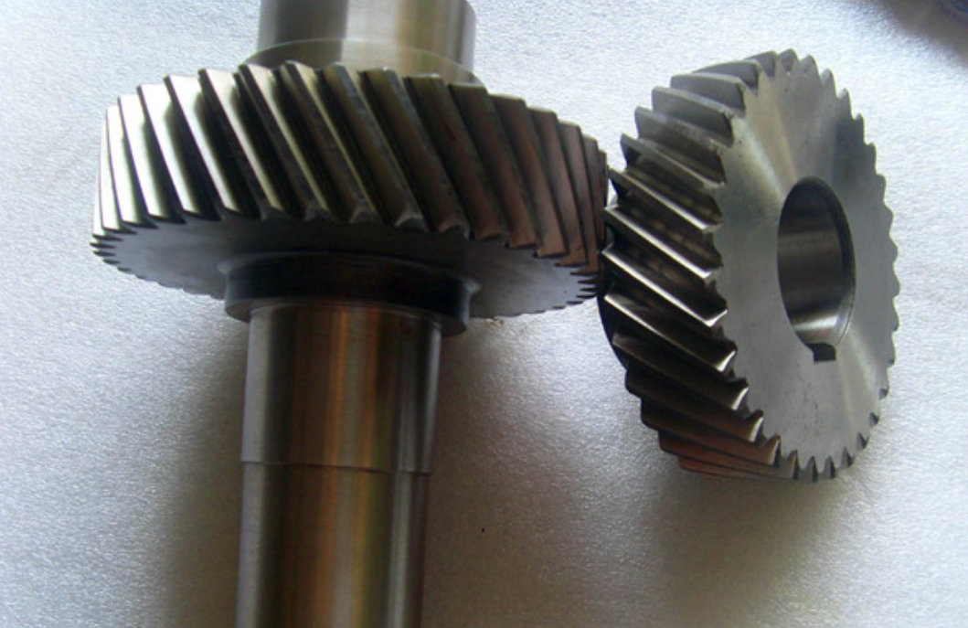
In modern mechanical transmission systems, helical gears play a pivotal role due to their superior load-bearing capacity, smooth operation, and reduced noise compared to spur gears. As a key component in applications such as automotive transmissions, industrial machinery, and aerospace systems, understanding the dynamic behavior of helical gears is essential for ensuring reliability and performance. Modal analysis, which investigates the natural frequencies and mode shapes of a structure, is a fundamental tool in this endeavor. It helps predict resonance conditions and vibrational tendencies, thereby guiding design improvements to avoid catastrophic failures. In this study, I explore the modal characteristics of a helical gear pair from a heavy-duty vehicle transmission using two distinct approaches: an analytical method based on a six-degree-of-freedom (6-DOF) dynamic model implemented in Matlab, and a finite element method (FEM) conducted in Ansys Workbench. By comparing these methodologies, I aim to validate the dynamic model, elucidate their respective advantages and limitations, and provide insights into the vibrational response of helical gears under operational conditions. The integration of Matlab’s robust numerical capabilities for dynamic response analysis further enriches this investigation, offering a holistic view of gear dynamics.
The helical gear system, as studied here, operates in a three-dimensional space where vibrations manifest in multiple directions, including translational movements along the tangential and axial axes, as well as rotational motions. To capture this complexity, I developed a lumped-parameter dynamic model with six degrees of freedom, encompassing four translational and two rotational DOFs. This model neglects frictional effects to simplify the analysis while retaining essential dynamic interactions. The figure below illustrates the meshing configuration of the helical gear pair, highlighting the coordinate system used for modeling.
Applying Newton’s second law, the equations of motion for the system can be derived. The dynamic model accounts for masses, moments of inertia, support stiffness and damping in tangential and axial directions, torsional stiffness, and the dynamic meshing forces generated during gear engagement. For the driving gear (denoted as gear 1) and the driven gear (gear 2), the displacements are defined as follows: $y_1$ and $y_2$ for tangential translations, $z_1$ and $z_2$ for axial translations, and $\theta_1$ and $\theta_2$ for rotational angles. The parameters include masses $m_1$ and $m_2$, moments of inertia $I_1$ and $I_2$, base circle radii $r_1$ and $r_2$, support stiffness coefficients $k_{1y}$, $k_{1z}$, $k_{2y}$, $k_{2z}$, support damping coefficients $c_{1y}$, $c_{1z}$, $c_{2y}$, $c_{2z}$, torsional stiffness $k_t$, input torque $T_1$, and load torque $T_2$. The dynamic meshing forces in the tangential and axial directions, $F_y$ and $F_z$, depend on the average meshing stiffness $k_m$, average meshing damping $c_m$, helix angle $\beta$, and transmission errors $e_y$ and $e_z$.
The system’s equations of motion are expressed as:
$$
\begin{aligned}
m_1 \ddot{y}_1 + c_{1y} \dot{y}_1 + k_{1y} y_1 &= -F_y, \\
m_1 \ddot{z}_1 + c_{1z} \dot{z}_1 + k_{1z} z_1 &= F_z, \\
I_1 \ddot{\theta}_1 + r_1 F_y + k_t \theta_1 &= -T_1, \\
m_2 \ddot{y}_2 + c_{2y} \dot{y}_2 + k_{2y} y_2 &= F_y, \\
m_2 \ddot{z}_2 + c_{2z} \dot{z}_2 + k_{2z} z_2 &= -F_z, \\
I_2 \ddot{\theta}_2 + r_2 F_y + k_t \theta_2 &= -T_2.
\end{aligned}
$$
The tangential and axial dynamic meshing forces are given by:
$$
F_y = k_m \cos\beta (y_1 + r_1 \theta_1 – y_2 – r_2 \theta_2 – e_y) + c_m \cos\beta (\dot{y}_1 + r_1 \dot{\theta}_1 – \dot{y}_2 – r_2 \dot{\theta}_2 – \dot{e}_y),
$$
$$
F_z = k_m \sin\beta [z_1 – z_2 – (y_1 + r_1 \theta_1 – y_2 – r_2 \theta_2) \tan\beta – e_z] + c_m \sin\beta [\dot{z}_1 – \dot{z}_2 – (\dot{y}_1 + r_1 \dot{\theta}_1 – \dot{y}_2 – r_2 \dot{\theta}_2) \tan\beta – \dot{e}_z].
$$
Substituting these forces into the equations of motion and assembling them in matrix form yields:
$$
[M]\{\ddot{\delta}\} + [C]\{\dot{\delta}\} + [K]\{\delta\} = \{F\},
$$
where the displacement vector is $\{\delta\} = \{y_1, z_1, \theta_1, y_2, z_2, \theta_2\}^T$. The mass matrix $[M]$ is diagonal, and the stiffness matrix $[K]$ and damping matrix $[C]$ are symmetric, reflecting the coupling between degrees of freedom due to the helical gear geometry. For modal analysis, damping and external forces are often neglected to focus on inherent characteristics. Thus, the free vibration equation reduces to:
$$
[M]\{\ddot{\delta}\} + [K]\{\delta\} = \{0\}.
$$
This formulation provides the foundation for analytical modal extraction via eigenvalue analysis.
To perform the analytical modal analysis, I first computed the necessary parameters for the helical gear pair based on its design specifications. Using Matlab, I programmed calculations for masses, moments of inertia, stiffness values, and other dynamic parameters. The helical gear parameters, such as module, number of teeth, face width, and helix angle, were derived from the heavy-duty transmission application. The material properties, including Young’s modulus and density, were also incorporated. The computed parameters are summarized in Table 1.
| Parameter | Symbol | Value | Unit |
|---|---|---|---|
| Mass of driving gear | $m_1$ | 6.108 | kg |
| Mass of driven gear | $m_2$ | 6.650 | kg |
| Moment of inertia (driving) | $I_1$ | 0.016 | kg·m² |
| Moment of inertia (driven) | $I_2$ | 0.020 | kg·m² |
| Base circle radius (driving) | $r_1$ | 0.07284 | m |
| Base circle radius (driven) | $r_2$ | 0.07927 | m |
| Tangential support stiffness (driving) | $k_{1y}$ | 1.95 × 10⁹ | N/m |
| Axial support stiffness (driving) | $k_{1z}$ | 0.75 × 10⁹ | N/m |
| Tangential support stiffness (driven) | $k_{2y}$ | 2.98 × 10⁹ | N/m |
| Axial support stiffness (driven) | $k_{2z}$ | 1.14 × 10⁹ | N/m |
| Average meshing stiffness | $k_m$ | 1.058 × 10⁹ | N/m |
| Torsional stiffness | $k_t$ | Assumed integrated in model | N·m/rad |
| Helix angle | $\beta$ | Based on design (e.g., 20°) | degrees |
With these parameters, I constructed the mass and stiffness matrices in Matlab. The eigenvalue problem was solved using the command eig(K, M), which yields the natural frequencies and mode shapes. The characteristic equation is:
$$
\det([K] – \omega^2 [M]) = 0,
$$
where $\omega$ represents the circular natural frequencies. The first six natural frequencies in Hz are listed in Table 2, obtained by converting $\omega$ to Hertz via $f = \omega / (2\pi)$.
| Mode Number | Natural Frequency (Hz) | Primary Vibration Direction |
|---|---|---|
| 1 | 1225 | Axial translation coupled with torsion |
| 2 | 1871 | Axial translation with phase opposition |
| 3 | 2965 | Tangential bending and torsion |
| 4 | 4622 | Strong torsional dominance |
| 5 | 8318 | High-frequency torsion |
| 6 | 9032 | Very high-frequency torsion |
The corresponding mode shapes, represented as eigenvectors, illustrate the relative displacements of each degree of freedom. For instance, the first mode shape predominantly involves axial movements of both gears, while higher modes exhibit increasing torsional components. These mode shapes are crucial for identifying potential resonance points and understanding the coupling between different vibration forms in helical gears.
Beyond modal analysis, I investigated the dynamic response of the helical gear system under operational conditions. Using Matlab’s ODE solvers, specifically the Runge-Kutta method (ode45), I simulated the time-domain response by solving the full differential equations with damping and excitation forces. The input conditions were set to mimic real-world operation: an input speed of 1500 rpm and an input torque of 200 N·m. The transmission errors $e_y$ and $e_z$ were modeled as sinusoidal functions to represent manufacturing imperfections. The dynamic response provides displacement histories for each degree of freedom, revealing the vibrational amplitudes during meshing.
The results indicate that the helical gear system exhibits significant vibrations, with the driven gear experiencing larger displacements than the driving gear. Key observations from the response analysis are quantified in Table 3, which summarizes the maximum displacements and angles.
| Degree of Freedom | Maximum Displacement (mm or degrees) | Notes |
|---|---|---|
| Driving gear tangential ($y_1$) | 0.150 mm | Moderate tangential vibration |
| Driving gear axial ($z_1$) | 0.013 mm | Minimal axial vibration |
| Driving gear torsion ($\theta_1$) | 0.400° | Equivalent to 0.36 mm at tooth tip |
| Driven gear tangential ($y_2$) | 0.200 mm | Higher than driving gear |
| Driven gear axial ($z_2$) | 0.012 mm | Negligible axial contribution |
| Driven gear torsion ($\theta_2$) | 0.800° | Equivalent to 1.31 mm at tooth tip |
These values demonstrate that torsional vibrations are the most pronounced, particularly for the driven helical gear, where the torsional displacement at the tooth tip exceeds 1 mm. Tangential vibrations are secondary but still considerable, while axial vibrations are minimal. This hierarchy underscores the importance of torsional stiffness in helical gear design and suggests that dynamic models should prioritize accurate representation of rotational inertia and stiffness.
To complement the analytical approach, I conducted a finite element modal analysis using Ansys Workbench. This method involves creating a detailed three-dimensional model of the helical gear pair, discretizing it into finite elements, and solving for eigenvalues and eigenvectors. The process begins with geometry modeling; I designed the helical gears in SolidWorks based on the same parameters used in the analytical model, ensuring consistency. The gears were then assembled with proper meshing alignment and imported into Workbench.
Material properties were assigned to reflect the typical alloy steel used in automotive transmissions, such as 20CrMnTi. The properties include a Young’s modulus of 210 GPa, a Poisson’s ratio of 0.3, and a density of 7850 kg/m³. These values are critical for accurate FEM results. The finite element mesh was generated using an automatic tetrahedral dominant method, which balances computational efficiency and accuracy. The mesh statistics are summarized in Table 4.
| Mesh Parameter | Value |
|---|---|
| Element Type | Quadratic tetrahedral (Solid 187) |
| Number of Nodes | Approximately 150,000 |
| Number of Elements | Approximately 90,000 |
| Mesh Quality | Skewness < 0.7, suitable for modal analysis |
Boundary conditions were applied to simulate realistic constraints: the gear hubs were fixed in all translational and rotational degrees of freedom except for the rotational axis, allowing free rotation. Contact between the helical gear teeth was defined as frictional with a coefficient of 0.2, though for linear modal analysis, contact stiffness is linearized. The Lanczos eigenvalue solver was employed to extract the first six natural frequencies and mode shapes. The results are presented in Table 5.
| Mode Number | Natural Frequency (Hz) | Mode Shape Description |
|---|---|---|
| 1 | 1197.5 | Bending of teeth in contact region |
| 2 | 1850.2 | Alternating tooth bending |
| 3 | 2948.7 | Combined tangential bending and torsion |
| 4 | 4601.4 | Dominant torsional vibration |
| 5 | 8305.9 | High-order torsion |
| 6 | 8903.3 | Very high-order torsion with axial coupling |
The mode shapes from FEM visually depict deformation patterns. For example, the first mode shows significant flexure at the meshing teeth, indicating susceptibility to bending stresses. The third mode involves both tangential displacements and rotational twists, highlighting the three-dimensional nature of helical gear vibrations. These visualizations, though not included here due to format constraints, reinforce the analytical findings and provide intuitive insights into gear dynamics.
Comparing the results from the analytical and finite element methods reveals both consistencies and discrepancies. Table 6 juxtaposes the natural frequencies obtained from both approaches, along with percentage differences.
| Mode Number | Analytical Frequency (Hz) | FEM Frequency (Hz) | Difference (%) |
|---|---|---|---|
| 1 | 1225 | 1197.5 | 2.24 |
| 2 | 1871 | 1850.2 | 1.11 |
| 3 | 2965 | 2948.7 | 0.55 |
| 4 | 4622 | 4601.4 | 0.45 |
| 5 | 8318 | 8305.9 | 0.15 |
| 6 | 9032 | 8903.3 | 1.43 |
The close agreement, with differences generally below 2.5%, validates the 6-DOF dynamic model as an effective representation of the helical gear system. Minor deviations arise from modeling assumptions: the analytical method uses lumped parameters and simplified stiffness values, whereas FEM accounts for distributed mass and stiffness through continuous discretization. Notably, FEM captures higher-mode details more accurately due to its finer spatial resolution, but at increased computational cost. Both methods confirm that the helical gear’s natural frequencies are well above the typical meshing frequency for this application (calculated as up to 1133 Hz at maximum speed), implying a low risk of resonance.
In terms of advantages, the analytical method offers rapid computation and deep insight into parametric influences, making it ideal for preliminary design and sensitivity studies. For instance, one can easily modify stiffness or mass values in Matlab to observe effects on natural frequencies. The dynamic response analysis further extends its utility for simulating transient behaviors. Conversely, FEM provides high accuracy and detailed stress-strain information, essential for fatigue life prediction and optimization of complex geometries. However, it requires significant preprocessing and computational resources. For helical gears, which involve intricate tooth profiles and three-dimensional forces, FEM is invaluable for capturing local effects like tooth root stresses and contact patterns.
To further explore the dynamics, I performed additional parametric studies using the analytical model. By varying key parameters such as helix angle, support stiffness, and meshing stiffness, I assessed their impact on modal properties. The relationship between helix angle $\beta$ and natural frequencies can be approximated by:
$$
\omega \propto \sqrt{\frac{k_m \cos^2\beta + k_{axial} \sin^2\beta}{m_{eq}}},
$$
where $m_{eq}$ is an equivalent mass. This shows that increasing the helix angle shifts energy between tangential and axial vibrations, potentially altering mode shapes. Such analyses underscore the versatility of the analytical approach for iterative design improvements.
In conclusion, this comprehensive study demonstrates the effectiveness of combining analytical and finite element methods for modal analysis of helical gears. The 6-DOF dynamic model, implemented in Matlab, provides a reliable foundation for understanding global vibrational characteristics, while FEM in Workbench offers refined insights into local deformations. Both methods highlight the predominance of torsional vibrations in helical gears, guiding designers to prioritize torsional stiffness in transmission systems. The dynamic response analysis further reveals operational displacement magnitudes, aiding in noise and vibration mitigation strategies. Future work could incorporate nonlinear factors, such as time-varying meshing stiffness and backlash, to enhance model fidelity. Ultimately, this integrated approach facilitates robust helical gear design, ensuring performance and durability across diverse engineering applications.