
In the field of gear transmission systems, the time-varying mesh stiffness of helical gears serves as a primary internal excitation source for vibrations and is fundamental to determining load distribution among teeth. Accurate and efficient calculation of this stiffness is crucial for dynamic analysis and strength assessment of helical gears. Traditional methods for computing mesh stiffness include the material mechanics method, finite element analysis, and approximate substitution approaches. However, each method has limitations: the material mechanics method, while fast, is not directly applicable to helical gears due to geometric complexities; finite element methods, though accurate, are computationally intensive; and approximate substitution methods, which simplify stiffness variation based on contact line length changes, may lack precision by ignoring variations in mesh stiffness per unit length during engagement. In this study, we develop a quasi-static elastic model for helical gears that integrates contact line length variation, a parabolic model for single-tooth mesh stiffness per unit length, and the ISO6336-1 standard. We compare this model with a quasi-static rigid model (an approximate substitution method) and ISO standards to validate accuracy. Furthermore, we analyze the influence of geometric parameters such as helix angle and tooth width on comprehensive mesh stiffness and load distribution coefficients. Additionally, we investigate the effects of typical broken tooth faults—specifically, failures along the contact line direction and along the tooth width direction—on mesh stiffness and load sharing. This research provides a foundational basis for fault dynamics studies in helical gear systems, enhancing the understanding of stiffness激励 and load distribution under both healthy and faulty conditions.
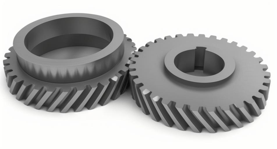
The engagement of helical gears involves continuous changes in contact lines due to their helical nature, leading to multiple tooth pairs meshing simultaneously at different positions along the tooth height. This complexity necessitates a detailed model to capture stiffness variations accurately. The quasi-static rigid model assumes uniform load distribution along the contact line and constant mesh stiffness per unit length, reducing stiffness calculation to a function of total contact line length. In contrast, the quasi-static elastic model accounts for non-uniform stiffness along the tooth profile by incorporating a parabolic distribution for single-tooth stiffness per unit length, derived from empirical studies. We begin by deriving the contact line length variation for helical gears. When the meshing plane is developed on the base circle, the dimensionless contact line length for a single tooth pair, denoted as \( l_0(\tau) \), can be expressed as a periodic linear function, where \( \tau = \mu / p_{bt} \) is the dimensionless meshing coordinate, \( \mu \) is the distance along the base circle projection, \( p_{bt} \) is the base pitch, and \( \varepsilon_\alpha \), \( \varepsilon_\beta \), and \( \varepsilon_\gamma \) are the transverse, axial, and total contact ratios, respectively. The function is given by:
$$ l_0(\tau) =
\begin{cases}
\tau / \min(\varepsilon_\alpha, \varepsilon_\beta), & \tau \leq \min(\varepsilon_\alpha, \varepsilon_\beta) \\
1, & \min(\varepsilon_\alpha, \varepsilon_\beta) < \tau \leq \max(\varepsilon_\alpha, \varepsilon_\beta) \\
(\varepsilon_\gamma – \tau) / \min(\varepsilon_\alpha, \varepsilon_\beta), & \max(\varepsilon_\alpha, \varepsilon_\beta) < \tau \leq \varepsilon_\gamma
\end{cases} $$
The total contact line length at any time, \( L(\tau) \), is the sum of lengths for all simultaneously engaged tooth pairs, calculated as \( L(\tau) = \sum_{i=0}^{N-1} l(\tau – \text{floor}(\tau) + i) \), where \( N \) is the number of tooth pairs in contact. In the quasi-static rigid model, the comprehensive mesh stiffness \( K_R(\tau) \) is proportional to \( L(\tau) \): \( K_R(\tau) = k_L L(\tau) \), with \( k_L \) being the mesh stiffness per unit length derived from ISO6336-1. The load distribution coefficient \( R \) for each tooth pair is then \( R = l_i(\tau) / L(\tau) \), where \( l_i(\tau) \) is the contact line length of the i-th pair.
For the quasi-static elastic model, we incorporate a parabolic model for single-tooth mesh stiffness per unit length, denoted as \( k_0(\tau) \), which varies with the meshing position. This model is expressed as:
$$ k_0(\tau) = \frac{4(\alpha_k – 1)}{\varepsilon_\gamma^2} \tau^2 – \frac{4(\alpha_k – 1)}{\varepsilon_\gamma} \tau + \alpha_k $$
Here, \( \alpha_k \) represents the ratio of minimum to maximum stiffness for a single tooth pair. Studies suggest that \( \alpha_k = 0.55 \) yields results consistent with ISO standards for helical gears. The single-tooth mesh stiffness \( k(\tau) \) is then \( k(\tau) = k_{\text{max}} l_0(\tau) k_0(\tau) \), where \( k_{\text{max}} \) is the maximum single-tooth stiffness from ISO6336-1. The comprehensive mesh stiffness \( K_E(\tau) \) is the sum of stiffnesses of all engaged pairs: \( K_E(\tau) = \sum_{i=0}^{N-1} k(\tau – \text{floor}(\tau) + i) \). Consequently, the load distribution coefficient becomes \( R = k_i(\tau) / K_E(\tau) \), reflecting the influence of stiffness variation on load sharing.
To validate our models, we compare calculations for a helical gear pair with parameters listed in Table 1. The gear pair has 16 and 107 teeth, a normal module of 5.5 mm, a normal pressure angle of 20°, a tooth width of 75 mm, and a helix angle of 17°. We compute mesh stiffness using both models for \( \alpha_k = 0.55 \) and \( \alpha_k = 0.8 \), and compare results with ISO6336-1 standards. Table 2 summarizes the mean comprehensive mesh stiffness values for different helix angles, highlighting percentage errors relative to ISO standards. The quasi-static elastic model with \( \alpha_k = 0.55 \) shows the best agreement, with errors below 4%, while the quasi-static rigid model exhibits errors exceeding 10%. This underscores the importance of accounting for stiffness per unit length variations in helical gears.
| Parameter | Symbol | Value |
|---|---|---|
| Number of teeth (pinion) | \( z_1 \) | 16 |
| Number of teeth (gear) | \( z_2 \) | 107 |
| Normal module | \( m_n \) | 5.5 mm |
| Normal pressure angle | \( \alpha_n \) | 20° |
| Tooth width | \( b \) | 75 mm |
| Helix angle | \( \beta \) | 17° |
| Model | Mean Stiffness for \( \beta = 9^\circ \) (10⁹ N/m) | Error (%) | Mean Stiffness for \( \beta = 13^\circ \) (10⁹ N/m) | Error (%) | Mean Stiffness for \( \beta = 17^\circ \) (10⁹ N/m) | Error (%) | Mean Stiffness for \( \beta = 21^\circ \) (10⁹ N/m) | Error (%) |
|---|---|---|---|---|---|---|---|---|
| ISO6336-1 | 1.513 | – | 1.498 | – | 1.478 | – | 1.420 | – |
| Quasi-static elastic model (\( \alpha_k = 0.55 \)) | 1.506 | -0.46 | 1.519 | 1.40 | 1.507 | 1.96 | 1.465 | 3.17 |
| Quasi-static elastic model (\( \alpha_k = 0.8 \)) | 1.588 | 4.96 | 1.594 | 6.41 | 1.577 | 6.70 | 1.531 | 7.82 |
| Quasi-static rigid model | 1.654 | 9.92 | 1.654 | 10.41 | 1.633 | 10.49 | 1.584 | 11.55 |
The influence of geometric parameters on helical gears’ mesh stiffness and load distribution is significant. We analyze helix angle \( \beta \) and tooth width \( b \) using the quasi-static elastic model with \( \alpha_k = 0.55 \). As the helix angle increases, the mean comprehensive mesh stiffness initially decreases and then rises, with minimal fluctuation observed at \( \beta = 13^\circ \). The load distribution coefficient peaks decrease with larger helix angles, resulting in flatter curves and more uniform load sharing. Similarly, increasing tooth width boosts mean stiffness but reduces fluctuation when \( b = 60 \) mm, as shown by the stiffness fluctuation factor \( \Delta = (K_{\text{max}} – K_{\text{min}}) / K_a \). This factor oscillates with changes in helix angle and tooth width, reaching minima when the axial contact ratio \( \varepsilon_\beta \) is an integer (e.g., 1 or 2), indicating smoother engagement. For instance, at \( \beta = 13^\circ \) or \( b = 60 \) mm, where \( \varepsilon_\beta \approx 1 \), stiffness fluctuations are minimized, optimizing gear performance. These findings highlight the role of parameter optimization in mitigating stiffness激励 in helical gears.
Broken tooth faults in helical gears drastically alter mesh stiffness and load distribution. We examine two typical fault models: breakage along the contact line direction (Model 1) and along the tooth width direction (Model 2). For Model 1, the reduction in contact line length \( \Delta l_{b1} \) depends on the breakage position \( \mu_{b1} \). When \( 0 < \mu_{b1} \leq \min(\varepsilon_\alpha, \varepsilon_\beta) p_{bt} \), the reduction is:
$$ \Delta l_{b1} =
\begin{cases}
\mu / \sin \beta_b, & \mu \leq \mu_{b1} \\
0, & \mu_{b1} < \mu \leq \varepsilon_\gamma p_{bt}
\end{cases} $$
For Model 2, with breakage position \( \mu_{b2} \), the reduction \( \Delta l_{b2} \) is more complex, extending over a larger meshing interval. When \( 0 < \mu_{b2} \leq \min(\varepsilon_\alpha, \varepsilon_\beta) p_{bt} \), it is given by:
$$ \Delta l_{b2} =
\begin{cases}
\mu / \sin \beta_b, & \mu \leq \mu_{b2} \\
\mu_{b2} / \sin \beta_b, & \mu_{b2} < \mu \leq \varepsilon_\beta p_{bt} \\
[(\varepsilon_\beta p_{bt} + \mu_{b2}) – \mu] / \sin \beta_b, & \varepsilon_\beta p_{bt} < \mu \leq (\varepsilon_\beta p_{bt} + \mu_{b2}) \\
0, & (\varepsilon_\beta p_{bt} + \mu_{b2}) < \mu \leq \varepsilon_\gamma p_{bt}
\end{cases} $$
The modified contact length for a faulty tooth pair is \( l_b(\mu) = l(\mu) – \Delta l_b(\mu) \). Using these models, we compute comprehensive mesh stiffness and load distribution coefficients for various breakage sizes. For breakage along the contact line, stiffness drops sharply within the fault region \( [0, \mu_{b1}] \), recovering immediately after. Load distribution coefficients become zero in this region, indicating complete load loss on the broken tooth. For breakage along the tooth width, the affected region expands to \( [0, \mu_{b2} + \varepsilon_\beta p_{bt}] \), causing a prolonged reduction in stiffness and load sharing. In the interval \( [\mu_{b2}, \mu_{b2} + \varepsilon_\beta p_{bt}] \), load distribution coefficients are significantly lower compared to Model 1, exacerbating dynamic imbalances. This analysis demonstrates that breakage along the tooth width direction has a more severe impact on helical gears’ operational stability.
In conclusion, our quasi-static elastic model for helical gears, with \( \alpha_k = 0.55 \), provides accurate calculations of time-varying mesh stiffness and load distribution, aligning well with ISO6336-1 standards. The quasi-static rigid model, while simpler, introduces substantial errors due to its neglect of stiffness per unit length variations. Geometric parameters such as helix angle and tooth width critically influence stiffness fluctuations and load sharing; optimizing these parameters, particularly to achieve integer axial contact ratios, can minimize激励 and enhance gear performance. Furthermore, broken tooth faults significantly degrade mesh stiffness and alter load distribution, with breakage along the tooth width direction posing greater risks than along the contact line. These insights form a foundation for advanced dynamics and fault diagnosis in helical gear systems, emphasizing the need for precise modeling in design and maintenance. Future work could extend this approach to include effects of lubrication, wear, and other fault types, further refining the understanding of helical gears’ complex behavior.
To deepen the analysis, we derive additional formulas for helical gears’ contact mechanics. The base helix angle \( \beta_b \) relates to the normal helix angle \( \beta \) via \( \tan \beta_b = \tan \beta \cos \alpha_t \), where \( \alpha_t \) is the transverse pressure angle. The transverse contact ratio \( \varepsilon_\alpha \) is calculated as \( \varepsilon_\alpha = \frac{\sqrt{r_{a1}^2 – r_{b1}^2} + \sqrt{r_{a2}^2 – r_{b2}^2} – a \sin \alpha_t}{p_{bt}} \), with \( r_a \) as tip radius, \( r_b \) as base radius, and \( a \) as center distance. The axial contact ratio \( \varepsilon_\beta \) is \( \varepsilon_\beta = \frac{b \tan \beta_b}{p_{bt}} \). These parameters are essential for determining contact line variations in helical gears. Moreover, the maximum single-tooth stiffness \( k_{\text{max}} \) from ISO6336-1 can be expressed as \( k_{\text{max}} = C_M C_R C_B \cdot k_0 \), where \( C_M \), \( C_R \), and \( C_B \) are correction factors for material, rim, and width, and \( k_0 \) is the basic stiffness per unit width. This standardization ensures consistency across gear designs.
For load distribution, we can formulate the dynamic load per tooth pair as \( F_i = K_E(\tau) \cdot \delta_i \), where \( \delta_i \) is the deflection at the i-th contact point. In faulty conditions, this deflection increases, leading to higher dynamic loads on remaining teeth. The total transmitted load \( F_n \) relates to torque \( T \) by \( F_n = \frac{T}{r_b \cos \beta_b} \). These equations highlight the interplay between stiffness, load, and geometry in helical gears. To summarize key relationships, Table 3 provides formulas for stiffness and load distribution coefficients under different models.
| Model | Comprehensive Mesh Stiffness | Load Distribution Coefficient |
|---|---|---|
| Quasi-static rigid model | \( K_R(\tau) = k_L L(\tau) \) | \( R = \frac{l_i(\tau)}{L(\tau)} \) |
| Quasi-static elastic model | \( K_E(\tau) = \sum_{i=0}^{N-1} k_{\text{max}} l_0(\tau_i) k_0(\tau_i) \) | \( R = \frac{k_{\text{max}} l_0(\tau_i) k_0(\tau_i)}{K_E(\tau)} \) |
| Broken tooth (Model 1) | \( K(\tau) = \sum_{\text{healthy}} k(\tau) + \sum_{\text{faulty}} k_b(\tau) \) | \( R = \frac{k_i(\tau)}{K(\tau)} \text{ for healthy, } 0 \text{ for faulty} \) |
| Broken tooth (Model 2) | Same as above, with extended fault region | Reduced \( R \) in fault region |
Regarding geometric parameter effects, we quantify stiffness fluctuation factor \( \Delta \) as a function of helix angle and tooth width. For helix angles, \( \Delta(\beta) \) can be approximated by \( \Delta(\beta) = A \sin(2\pi \varepsilon_\beta) + B \), where \( A \) and \( B \) are constants derived from simulation data. This sinusoidal pattern reflects the periodic nature of contact line changes in helical gears. Similarly, for tooth width, \( \Delta(b) \) follows a trend where minima occur at \( b = n \cdot p_{bt} / \tan \beta_b \) for integer \( n \), corresponding to integer \( \varepsilon_\beta \). These relationships aid in designing helical gears with minimal vibration. For instance, selecting a helix angle of 13° or a tooth width of 60 mm for our example gear pair reduces \( \Delta \) to below 0.05, indicating smooth operation.
In fault analysis, the severity of breakage can be measured by the stiffness reduction ratio \( \rho = K_{\text{faulty}} / K_{\text{healthy}} \). For Model 1, \( \rho \) drops linearly with \( \mu_{b1} \), whereas for Model 2, \( \rho \) decreases more steeply due to the larger affected area. The load imbalance caused by faults increases dynamic loads on adjacent teeth, potentially leading to further failures. We calculate the increased load on neighboring teeth as \( F_{\text{neighbor}} = F_n / (1 – \zeta) \), where \( \zeta \) is the fraction of load lost from the broken tooth. For helical gears with high contact ratios, this effect is mitigated by multiple tooth engagement, but in cases of severe breakage, it remains a critical concern.
Our study underscores the importance of accurate stiffness modeling for helical gears in both healthy and faulty states. The quasi-static elastic model, validated against ISO standards, offers a reliable tool for predicting mesh stiffness and load distribution. By analyzing geometric parameters, we identify optimal design choices to enhance performance. Furthermore, understanding broken tooth effects provides insights for condition monitoring and maintenance strategies. Helical gears, with their complex engagement patterns, require detailed analysis to ensure reliability in applications such as automotive transmissions, wind turbines, and industrial machinery. Future research could integrate this model into full dynamic simulations, incorporating factors like thermal effects and surface roughness, to further advance the design and diagnosis of helical gear systems.