
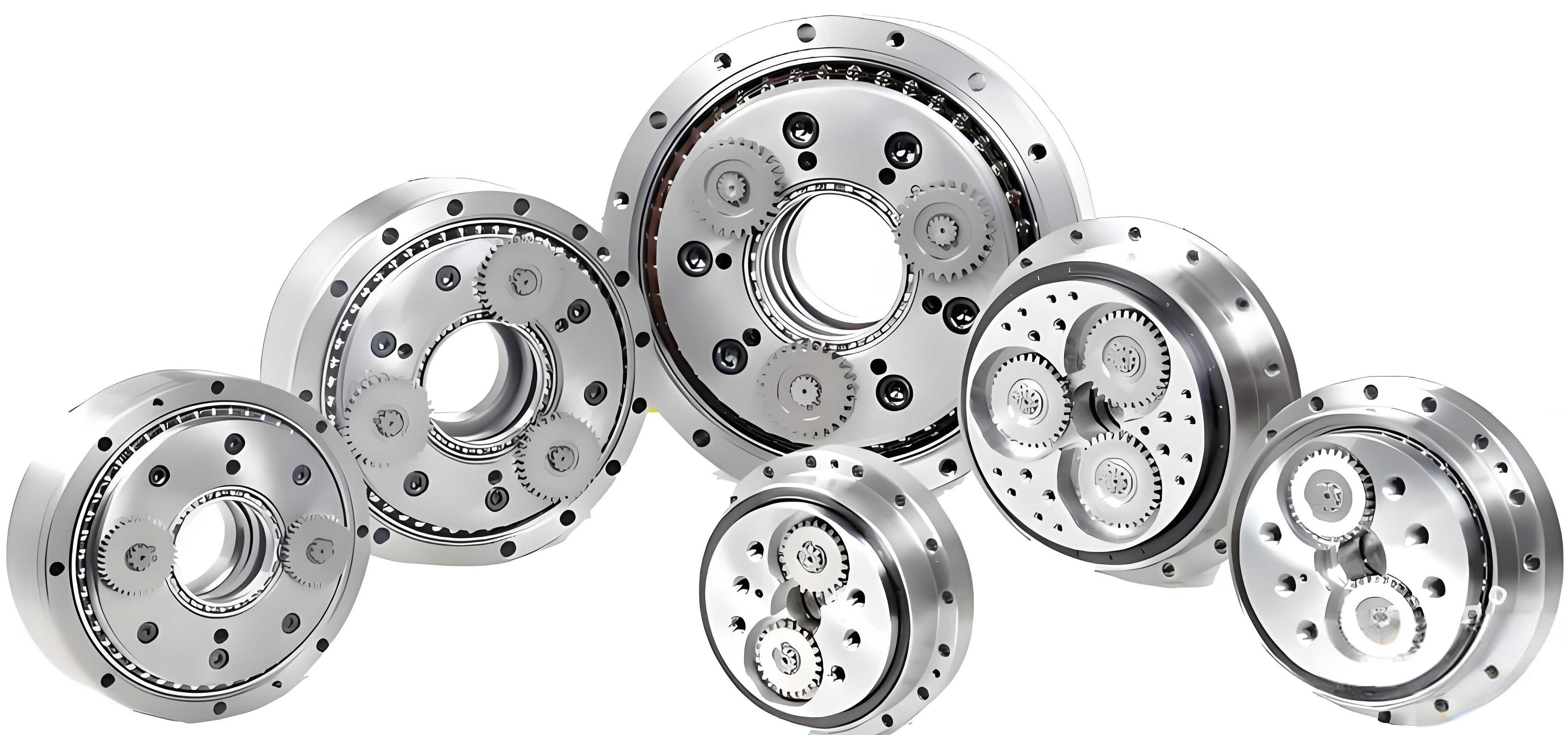
In the field of industrial robotics, the precision of transmission components is paramount, and the rotary vector reducer stands as a critical element in joint applications. The rotary vector reducer, often abbreviated as RV reducer, combines a primary planetary gear stage with a secondary cycloidal-pin gear stage, offering high transmission efficiency, stability, load capacity, compactness, and longevity. However, achieving and maintaining high transmission accuracy is challenging due to deviations introduced during manufacturing and assembly. This paper explores the transfer of deviations in rotary vector reducers under static assembly conditions using directed graph methodologies. We analyze deviation sources, categorize them, and develop models to represent deviation relationships and interactions between parts. The effectiveness of this approach is demonstrated through a case study on an RV320S-type rotary vector reducer, providing insights into how cumulative deviations impact transmission precision.
The rotary vector reducer is a key component in robotic joints, and its transmission accuracy has been a focal point of research. Deviations from ideal geometries and assembly processes inevitably affect performance, making it essential to understand deviation propagation. In static assembly, deviations arise from part dimensions, geometric tolerances, and assembly sequences. We classify these into three main types: geometric position deviations (E1), geometric form deviations (E2), and assembly position deviations (E3). Geometric position deviations include locational errors like diameter size deviations and coaxiality errors, as well as orientational errors like parallelism and perpendicularity deviations. Geometric form deviations encompass flatness, cylindricity, and straightness errors. Assembly position deviations stem from clamping, positioning, and clearance fits during assembly. These deviations couple and accumulate, ultimately influencing the transmission accuracy of the rotary vector reducer.
To model deviation transfer, we employ directed graphs, which visually represent relationships between parts and their deviations. In a rotary vector reducer, deviations propagate through two primary mechanisms: geometric coupling (Ha) and assembly clearance effects (Hb). Geometric coupling occurs when parts contact and their deviations interact, leading to cumulative effects downstream. In contrast, assembly clearance can interrupt deviation propagation, causing reset at certain interfaces. We define basic deviation flow models to capture these interactions. For instance, let \( g_{ij} \) denote the geometric feature \( j \) on part \( i \), and \( d_x \) represent a deviation source model, where \( x \geq 0 \). The coupling of deviations can be expressed as a directed edge from \( d_x \) to \( g_{ij} \), illustrating how deviations influence part geometries. For assembly position deviations, such as \( d_{13} \) for part 1, they couple with other deviation sources like \( d_0 \) to affect subsequent geometries like \( g_{21} \). This formalism allows us to trace deviation paths through the rotary vector reducer assembly.
We further develop directed graph models for fits and their deviations. In a rotary vector reducer, common fits include shaft-hole fits and surface-surface fits, such as gear meshing. For a shaft-hole fit, the constrained geometries are a shaft and a hole, each subject to deviation sources from their respective parts. Similarly, surface-surface fits involve two planes. The directed graph model for a fit includes nodes for the geometries \( g_{10} \) and \( g_{20} \), with deviation sources \( d_{11} \) to \( d_{1i} \) and \( d_{21} \) to \( d_{2j} \) influencing them. The coupling deviation \( d_0 \) represents the fit deviation itself. This model helps quantify how part deviations combine to affect fit quality and overall assembly accuracy in the rotary vector reducer.
For a concrete example, we consider the RV320S-type rotary vector reducer, which includes components like input shaft, sun gear, planet gears, crank shafts, bearings, cycloidal gears, pin sleeves, pin shafts, and output disk. We list the deviation types for each part based on our classification. Table 1 summarizes these deviations, highlighting how each part contributes to overall error. The rotary vector reducer’s complexity means deviations can accumulate across multiple stages, particularly from the crank shaft to the cycloidal gear and output disk.
| Component | Geometric Position Deviations (E1) | Geometric Form Deviations (E2) | Assembly Position Deviations (E3) |
|---|---|---|---|
| Input Shaft | Diameter size deviation, coaxiality with sun gear | Cylindricity, circular runout | Shaft-hole fit deviation with sun gear |
| Sun Gear | Diameter size deviation, coaxiality with input shaft, perpendicularity and parallelism | Profile tolerance | Shaft-hole fit with input shaft, gear mesh with planet gears |
| Planet Gear | Diameter size deviation, coaxiality with crank shaft, perpendicularity and parallelism | Profile tolerance | Shaft-hole fit with crank shaft, gear mesh with sun gear |
| Crank Shaft | Diameter size deviation, coaxiality with input shaft | Cylindricity, circular runout | Shaft-hole fit with planet gears |
| Bearing I | Coaxiality with crank shaft | Cylindricity, circular runout | Shaft-hole fit with crank shaft |
| Cycloidal Gear | Diameter size deviation, coaxiality with crank shaft, perpendicularity and parallelism | Profile tolerance | Clearance fit with bearings |
| Pin Sleeve | Coaxiality with pin shaft | Cylindricity, circular runout | Surface fit with cycloidal gear |
| Pin Shaft | Diameter size deviation | Cylindricity, circular runout | Shaft-hole fit with pin sleeve |
| Bearing II | Coaxiality with output disk | Cylindricity, circular runout | Clearance fit with cycloidal gear |
| Output Disk | Diameter size deviation, coaxiality with input shaft and crank shaft | Cylindricity, circular runout | Shaft-hole fit with bearing II |
Next, we analyze the fits between components in the rotary vector reducer. Table 2 details each fit, including the fit type, geometries involved, part numbers, and associated deviation codes. For example, the shaft-hole fit between the input shaft and sun gear (m1) involves geometries \( g_{11} \) and \( g_{21} \), with deviations \( E_{111} \) and \( E_{211} \). These deviations are typically size tolerances, such as \( P1 = 0_{-0.01} \) for the input shaft diameter and \( P2 = 0.01_0 \) for the sun gear bore. Similarly, gear meshes like between sun gear and planet gear (m2) are modeled as surface-surface fits with profile deviations. The rotary vector reducer’s performance hinges on these fits, as deviations here directly affect backlash and transmission error.
| Fit Interface | Fit Type and Code | Geometry and Code | Component Numbers | Deviation Codes |
|---|---|---|---|---|
| Input Shaft-Sun Gear | Shaft-hole fit, m1 | \( g_{11} \), \( g_{21} \) | p1, p2 | \( E_{111} \), \( E_{211} \) |
| Sun Gear-Planet Gear | Surface-surface fit, m2 | \( g_{22} \), \( g_{32} \) | p2, p3 | \( E_{221} \), \( E_{321} \) |
| Planet Gear-Crank Shaft | Shaft-hole fit, m3 | \( g_{31} \), \( g_{41} \) | p3, p4 | \( E_{311} \), \( E_{411} \) |
| Crank Shaft-Bearing I | Shaft-hole fit, m4 | \( g_{41} \), \( g_{51} \) | p4, p5 | \( E_{411} \), \( E_{511} \) |
| Bearing I-Cycloidal Gear | Surface-surface fit, m5 | \( g_{52} \), \( g_{61} \) | p5, p6 | \( E_{521} \), \( E_{611} \) |
| Cycloidal Gear-Pin Sleeve | Surface-surface fit, m6 | \( g_{62} \), \( g_{72} \) | p6, p7 | \( E_{621} \), \( E_{721} \) |
| Pin Sleeve-Pin Shaft | Shaft-hole fit, m7 | \( g_{71} \), \( g_{81} \) | p7, p8 | \( E_{711} \), \( E_{811} \) |
| Cycloidal Gear-Bearing II | Surface-surface fit, m8 | \( g_{63} \), \( g_{92} \) | p6, p9 | \( E_{631} \), \( E_{921} \) |
| Bearing II-Output Disk | Shaft-hole fit, m9 | \( g_{91} \), \( g_{101} \) | p9, p10 | \( E_{911} \), \( E_{1011} \) |
Assembly position requirements are crucial for the rotary vector reducer’s alignment. Table 3 lists these requirements, such as the coaxiality between the sun gear axis and input shaft axis. Each requirement is defined by functional and datum geometries, with deviation codes like \( E_{210} \) for the sun gear axis relative to the input shaft axis. These requirements ensure that parts are correctly positioned during assembly, minimizing cumulative errors. The rotary vector reducer’s transmission accuracy depends heavily on meeting these requirements, as misalignments can amplify deviations through the gear train.
| Position Requirement | Functional Geometry | Datum Geometry | Deviation Code |
|---|---|---|---|
| Sun gear axis relative to input shaft axis | \( g_{20} \) | \( g_{10} \) | \( E_{210} \) |
| Planet gear axis relative to sun gear axis | \( g_{30} \) | \( g_{20} \) | \( E_{320} \) |
| Crank shaft axis relative to planet gear axis | \( g_{40} \) | \( g_{30} \) | \( E_{430} \) |
| Bearing I axis relative to crank shaft axis | \( g_{50} \) | \( g_{40} \) | \( E_{540} \) |
| Cycloidal gear axis relative to bearing I axis | \( g_{60} \) | \( g_{50} \) | \( E_{650} \) |
| Pin sleeve axis relative to cycloidal gear axis | \( g_{70} \) | \( g_{60} \) | \( E_{760} \) |
| Pin shaft axis relative to pin sleeve axis | \( g_{80} \) | \( g_{70} \) | \( E_{870} \) |
| Bearing II axis relative to cycloidal gear axis | \( g_{90} \) | \( g_{60} \) | \( E_{960} \) |
| Output disk axis relative to bearing II axis | \( g_{100} \) | \( g_{90} \) | \( E_{1090} \) |
| Output disk axis relative to crank shaft axis | \( g_{100} \) | \( g_{40} \) | \( E_{1040} \) |
| Output disk axis relative to input shaft axis | \( g_{100} \) | \( g_{10} \) | \( E_{1010} \) |
Building on these tables, we construct a comprehensive deviation transfer directed graph model for the rotary vector reducer. This model integrates all deviation sources, fits, and position requirements into a single graph. Nodes represent part geometries and deviation sources, while edges indicate deviation propagation paths. For example, deviation from the input shaft \( E_{111} \) flows to the fit m1, coupling with \( E_{211} \) from the sun gear, then to the sun gear axis \( g_{20} \), and so on through the assembly. The directed graph visually shows that the most critical accumulation path is from the crank shaft through the cycloidal gear to the output disk. This accumulation significantly impacts the transmission accuracy of the rotary vector reducer. The model can be represented mathematically using adjacency matrices or flow equations. Let \( D \) be the vector of deviation sources, and \( G \) the vector of geometric features. The transfer can be modeled as \( G = T \cdot D \), where \( T \) is a transfer matrix derived from the directed graph. For instance, for a simple chain, the cumulative deviation \( \Delta G \) at the output is:
$$ \Delta G = \sum_{i=1}^{n} T_i \cdot D_i $$
where \( T_i \) are transfer coefficients representing the influence of deviation \( D_i \) on \( G \). In a rotary vector reducer, these coefficients depend on fit types and geometric relationships. For shaft-hole fits, the transfer might involve clearance effects, modeled as:
$$ T_{\text{shaft-hole}} = \frac{1}{1 + \delta_c} $$
where \( \delta_c \) is the clearance deviation. For gear meshes, transfer coefficients relate to contact ratios and pressure angles. The overall model allows us to simulate deviation accumulation and identify sensitivity points in the rotary vector reducer.
The directed graph model for the RV320S-type rotary vector reducer reveals several insights. First, deviations in the cycloidal gear stage (secondary transmission) have a disproportionate effect on output accuracy, consistent with prior research. This is because the cycloidal gear involves multiple contacts with pin sleeves, and small deviations can amplify due to the trochoidal motion. Second, assembly position deviations at clearance fits, such as between bearings and the cycloidal gear, can reset deviation chains, but also introduce randomness that complicates prediction. Third, the model highlights the importance of controlling coaxiality and parallelism in the crank shaft and bearing assemblies to reduce cumulative error. By quantifying these effects, we can prioritize tolerance design and assembly processes for the rotary vector reducer.
To validate the model, we consider a numerical example. Suppose the input shaft has a diameter deviation of \( \pm 0.005 \) mm, and the sun gear bore has a deviation of \( \pm 0.003 \) mm. The shaft-hole fit deviation \( d_0 \) for m1 can be calculated as the combined effect:
$$ d_0 = \sqrt{E_{111}^2 + E_{211}^2} $$
assuming independent normal distributions. For \( E_{111} = 0.005 \) and \( E_{211} = 0.003 \), we get \( d_0 \approx 0.0058 \) mm. This deviation then propagates to the sun gear axis \( g_{20} \), affecting subsequent meshes. Similarly, for gear meshes, profile deviations \( E_{221} \) and \( E_{321} \) couple to cause transmission error. The overall output deviation \( \Delta \theta \) at the output disk can be estimated by summing contributions along the graph paths. For the rotary vector reducer, a simplified formula might be:
$$ \Delta \theta = K_1 \cdot \Delta_{\text{primary}} + K_2 \cdot \Delta_{\text{secondary}} $$
where \( \Delta_{\text{primary}} \) and \( \Delta_{\text{secondary}} \) are deviations from the planetary and cycloidal stages, respectively, and \( K_1, K_2 \) are constants derived from gear ratios. Typically, \( K_2 > K_1 \), emphasizing the cycloidal stage’s sensitivity. This aligns with our directed graph showing strong accumulation in the secondary stage.
In practice, the directed graph model can be implemented in software for tolerance analysis of rotary vector reducers. Tools like MATLAB or Python can parse the graph structure, compute cumulative deviations using Monte Carlo simulations, and optimize tolerances to meet accuracy targets. For instance, we can define cost functions that balance manufacturing cost (tighter tolerances are expensive) against performance loss from deviations. The model also aids in root cause analysis; if a rotary vector reducer exhibits excessive backlash, the directed graph can trace it to specific deviation sources, such as pin sleeve wear or bearing clearance.
Beyond static assembly, dynamic effects in rotary vector reducers, such as load-induced deformations and thermal expansion, can interact with geometric deviations. Future work could extend the directed graph to include these factors, making it a comprehensive tool for precision design. However, even in static conditions, our model provides a foundation for understanding deviation transfer. The rotary vector reducer’s complexity demands such systematic approaches to achieve the high accuracy required in robotics.
In conclusion, the study of deviation transfer in rotary vector reducers using directed graphs offers a powerful methodology for precision engineering. We classified deviation sources into geometric position, geometric form, and assembly position types, and developed basic deviation flow models and fit models. Through the RV320S-type rotary vector reducer case, we constructed a detailed directed graph that visualizes deviation accumulation, particularly in the cycloidal stage. This model validates the effectiveness of directed graphs in analyzing assembly deviations and provides insights for tolerance design and assembly process improvement. The rotary vector reducer’s transmission accuracy is critically influenced by cumulative deviations, and our approach helps mitigate these effects, contributing to the advancement of high-performance robotic systems.
The implications of this research extend to other precision gear systems, but the rotary vector reducer remains a focal point due to its widespread use in industrial robots. By leveraging directed graphs, manufacturers can enhance quality control, reduce rework, and optimize costs while maintaining high accuracy. As robotics continues to evolve, the demand for reliable rotary vector reducers will only grow, making such analytical tools indispensable. We encourage further exploration into dynamic and thermal models to fully capture the behavior of rotary vector reducers in operational environments.