
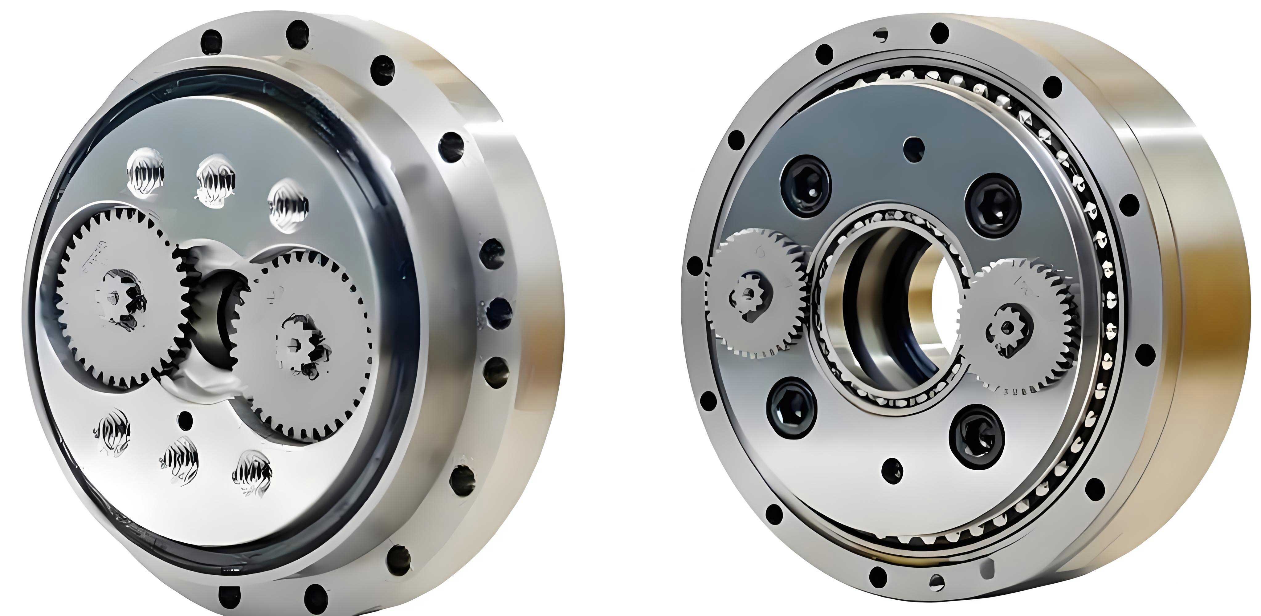
In the realm of precision machinery and industrial robotics, the rotary vector reducer stands as a pivotal component, often serving as the core transmission element within robotic joints. Its design, characterized by multiple tooth meshing simultaneously, grants it exceptional advantages such as high transmission ratio, remarkable precision, superior transmission efficiency, compact size, lightweight construction, high rigidity, and significant overload resistance. Consequently, the rotary vector reducer finds extensive applications across various fields including industrial manipulators, precision machine tools, assembly devices, and material handling systems. Despite its widespread adoption and mature development, research pertaining to the lifespan of rotary vector reducers remains relatively scarce. The operational life of a rotary vector reducer is a critical factor influencing its overall reliability, yet there exists a notable absence of universally effective calculation and verification methodologies. This article, from our research perspective, delves into the theoretical foundations and experimental validation of life estimation for these complex reducers, aiming to bridge this gap.
The pursuit of longevity and reliability in mechanical systems has always been paramount. For conventional power transmission components like spur gear reducers or worm gear drives, life prediction models and testing standards are well-established. However, the intricate architecture and high precision inherent to the rotary vector reducer present unique challenges for lifespan assessment. Its complexity arises from the integration of planetary gear stages and a cycloidal pin gear mechanism, leading to numerous interacting components under dynamic loads. Therefore, a focused study on the life calculation and accelerated testing of rotary vector reducers is not only necessary but also urgent for advancing their application in critical, high-reliability scenarios.
Our investigation begins with a theoretical analysis rooted in fundamental fatigue principles. The operational lifespan of any mechanical component subjected to cyclic loading is governed by material fatigue behavior. For the rotary vector reducer, the stresses experienced by its internal parts are not constant but fluctuate based on operational conditions. To model this, we turn to the well-established S-N fatigue theory, which describes the relationship between the cyclic stress amplitude (S) and the number of cycles to failure (N). This relationship is typically power-law in nature for the finite life region. The S-N curve illustrates that as the applied stress decreases, the number of cycles a component can endure increases dramatically, until a stress limit is reached below which the life can be considered infinite (or corresponds to a very high cycle count, \(N_0\)). Mathematically, this is expressed as:
$$ \sigma^m N = \text{constant} $$
where \(\sigma\) is the stress and \(m\) is an exponent dependent on the material and geometry. Since stress is proportional to applied force \(F\) or torque \(T\) in many mechanical elements, we can derive analogous relationships:
$$ F^{m’} N = C $$
$$ T^{m’} N = C $$
Here, \(m’\) is a related exponent, and \(C\) is a constant. For variable loading conditions, the equivalence between different load levels and their corresponding cycle counts can be established:
$$ \left( \frac{F_i}{F_j} \right) = \sqrt[m’]{\frac{N_j}{N_i}} \quad \text{for} \quad i, j = 1, 2, 3, \ldots, n \ (i \ne j) $$
$$ \left( \frac{T_i}{T_j} \right) = \sqrt[m’]{\frac{N_j}{N_i}} $$
These formulations are crucial for analyzing the rotary vector reducer under non-steady operational profiles.
To handle the cumulative damage under spectrum loading, we employ Miner’s linear damage rule (Miner’s theory). This rule posits that failure occurs when the sum of the cycle ratios for each stress level equals unity. In essence, the total energy absorbed by the component up to its fatigue limit is constant. If a component experiences stress levels \(\sigma_1, \sigma_2, \ldots, \sigma_n\) for \(n’_1, n’_2, \ldots, n’_n\) cycles respectively, and the cycles to failure at those stress levels are \(N_1, N_2, \ldots, N_n\), then Miner’s rule states:
$$ \sum_{i=1}^{n} \frac{n’_i}{N_i} = 1 $$
Combining this with the power-law relation from the S-N curve, and selecting a reference rated stress \(\sigma_0\) (corresponding to rated load \(F_0\) or rated torque \(T_0\)) with a reference life \(N_0\), we derive:
$$ \sigma_0^m N_0 = \sum_{i=1}^{n} \sigma_i^m n’_i $$
$$ N_0 = \sum_{i=1}^{n} \left( \frac{F_i}{F_0} \right)^{m’} n’_i $$
or
$$ N_0 = \sum_{i=1}^{n} \left( \frac{T_i}{T_0} \right)^{m’} n’_i $$
This forms the bedrock for predicting the life of mechanical systems under variable loads, including the sophisticated rotary vector reducer.
The total number of cycles \(N\) is related to the operating time \(t\) and rotational speed \(n\). For a constant speed \(n\), we have \(N = n t\). Substituting this into the torque-based Miner’s equation and considering a constant torque condition, we can derive a basic life formula for the reducer. If the rotary vector reducer operates under a constant torque \(T_i\) and speed \(n_i\), its life \(t_i\) relative to a rated life \(t_0\) at rated torque \(T_0\) and rated speed \(n_0\) is:
$$ t_i = t_0 \times \frac{n_0}{n_i} \times \left( \frac{T_0}{T_i} \right)^p $$
where \(p\) is a constant exponent to be determined. This is the fundamental life calculation formula. However, for practical application to a real-world rotary vector reducer, this formula requires refinement to account for various operational and environmental factors that significantly influence longevity.
In practice, the performance and lifespan of a rotary vector reducer are affected by multiple operational condition factors such as lubrication quality, load distribution, operating temperature, shaft stiffness, type of loading, and thermal gradients. Currently, there is a lack of specific research on condition coefficients for rotary vector reducers. Therefore, we adapt insights from bearing life calculation standards. Lubrication plays a vital role; an adequate lubricant film that separates surfaces minimizes wear and removes heat. When lubrication is optimal, a condition factor \(\alpha\) of 1.0 can be used. However, under less ideal circumstances—such as very low rotational speeds (e.g., below 10 rpm), insufficient lubricant viscosity at operating temperature, or elevated surface temperatures (e.g., above 40°C)—a factor \(\alpha\) of 0.9 is more appropriate. Incorporating this, the modified life formula for a rotary vector reducer becomes:
$$ t_i = t_0 \times \frac{n_0}{n_i} \times \left( \frac{T_0}{T_i} \right)^p \times \alpha $$
where \(\alpha\) is either 0.9 or 1.0 based on the assessed operating conditions.
The next critical step is to determine the exponent \(p\) and the rated life constant \(t_0\) specifically for the rotary vector reducer. Through analysis and testing, it has been observed that the life of the entire reducer assembly is often dominated by the fatigue life of its most critically stressed components. In the complex architecture of a rotary vector reducer, several bearing types are employed: angular contact ball bearings, tapered roller bearings, and needle roller bearings. Force analysis and failure mode studies indicate that the bearings mounted on the crankshaft—specifically the tapered roller bearings and, even more critically, the needle roller bearings—have a paramount influence on the overall system life. The needle roller bearings are typically installed in pairs on the crankshaft, positioned between the tapered roller bearings. These bearings are often non-standard, small in size, difficult to manufacture, and prone to failure. Therefore, we posit that the life of the rotary vector reducer can be effectively estimated based on the calculated life of these needle roller bearings.
To calculate the life of the needle roller bearing, we refer to the international standard ISO 281. The basic rating life \(L_{10}\) for a roller bearing (where the subscript 10 denotes 10% probability of failure, or 90% reliability) is given by:
$$ L_{10} = \frac{10^6}{60 n’} \left( \frac{C_r}{P_r} \right)^{10/3} $$
Here, \(L_{10}\) is the life in hours, \(n’\) is the bearing rotational speed in rpm, \(C_r\) is the basic dynamic load rating of the bearing in Newtons, and \(P_r\) is the equivalent dynamic radial load in Newtons. The exponent \(10/3\) is standard for roller bearings. The dynamic load rating \(C_r\) for a needle roller bearing can be calculated using the formula:
$$ C_r = b_m f_c (i L_{we} \cos\alpha)^{7/9} Z^{3/4} D_{we}^{29/27} $$
The parameters in this formula are defined in the following table:
| Symbol | Description | Typical Value/Note |
|---|---|---|
| \(b_m\) | Material and manufacturing process factor | 1.1 for roller bearings |
| \(f_c\) | Geometry factor | Depends on bearing geometry; obtained from reference tables based on pitch diameter. |
| \(i\) | Number of rows of rollers | Usually 1 for needle bearings in this application. |
| \(\alpha\) | Nominal contact angle | 0° for radial needle roller bearings. |
| \(L_{we}\) | Effective length of the roller | Measured in mm. |
| \(Z\) | Number of rollers | Count of needle rollers in the bearing. |
| \(D_{we}\) | Diameter of the roller | Measured in mm. |
The radial load \(P_r\) (equivalent to \(F_r\) in our earlier notation) acting on the needle roller bearing must be determined from the internal forces within the rotary vector reducer. Based on force analysis of the cycloidal gear’s bearing holes and applying action-reaction principles, the radial force on the needle bearing can be related to the output torque of the reducer. The relationship is:
$$ F_r = \frac{1}{M} \times \frac{T_m}{R} \times 1000 $$
where \(F_r\) is the radial force on the needle bearing in Newtons, \(T_m\) is the output torque of the rotary vector reducer in Newton-meters, \(R\) is the distance from the center of the cycloidal gear to the center of its bearing hole in millimeters, and \(M\) is a structural constant: for reducer models like 20E and 40E, \(M=4\); for 80E and larger, \(M=6\).
The rotational speed of the bearing \(n’\) is related to the output speed of the rotary vector reducer \(n\) by the transmission ratio. For a standard rotary vector reducer, this ratio is typically high (e.g., 40:1 or higher). Therefore, \(n’ = i_r \times n\), where \(i_r\) is the speed multiplication factor from output to the crankshaft (often equal to the first-stage reduction ratio). Considering the transmission efficiency \(\eta\) of the rotary vector reducer, the effective load on the bearing for life calculation may also be adjusted. Combining these elements, the life formula for the needle roller bearing becomes:
$$ L_{10h} = \frac{10^6}{60 \times (i_r \cdot n)} \left( \frac{C_r \cdot \eta}{ \frac{1}{M} \cdot \frac{T_m}{R} \cdot 1000 } \right)^{10/3} $$
Given that the life of the rotary vector reducer is constrained by this critical bearing, we equate the exponent \(p\) in our general reducer life formula to the roller bearing exponent \(10/3\). Furthermore, we can define the rated life constant \(K_0\) (equivalent to \(t_0\) at rated conditions) from this bearing life calculation at rated torque \(T_0\) and rated speed \(n_0\). Thus, the proposed comprehensive life formula for a rotary vector reducer, operating under average conditions defined by average output torque \(T_a\) and average output speed \(n_a\), is:
$$ L_h = K_0 \times \frac{n_0}{n_a} \times \left( \frac{T_0}{T_a} \right)^{10/3} \times \alpha $$
In this formula:
- \(L_h\) is the estimated life in hours with 90% reliability for the rotary vector reducer.
- \(K_0\) is the rated life constant in hours, which can be initially taken as 6000 hours based on common manufacturer specifications, but should be derived from detailed bearing analysis for accuracy.
- \(n_0\) is the rated output speed (rpm).
- \(T_0\) is the rated output torque (Nm).
- \(n_a\) is the average output speed during operation (rpm).
- \(T_a\) is the average output torque during operation (Nm).
- \(\alpha\) is the operating condition factor (0.9 or 1.0).
This equation highlights the inverse power relationship between torque and life, and the direct influence of speed. It provides a practical tool for estimating the lifespan of a rotary vector reducer under specified duty cycles.
To demonstrate the application of this life calculation methodology, we perform an example calculation for a specific rotary vector reducer model, which we refer to as the RV-40E-121 type. The key parameters for this reducer, as might be provided by a manufacturer, are summarized below:
| Parameter Name | Value |
|---|---|
| Model | RV-40E-121 |
| Rated Speed, \(n_0\) | 15 rpm |
| Rated Torque, \(T_0\) | 412 Nm |
| Maximum Allowable Moment | 1666 Nm |
| Allowable Start/Stop Torque | 1029 Nm |
| Maximum Speed | 70 rpm |
| Backlash (Max) | 1 arc-min |
| Moment of Inertia | 1.43 kg·m² |
| Spring Constant | 108 Nm/arc-min |
| Mass | 9.3 kg |
For the life calculation, we focus on the critical needle roller bearing. First, the radial force on the bearing under rated torque is computed. The distance \(R\) (from cycloidal gear center to bearing hole center) is measured as 36 mm for this 40E model. Using the force formula with \(M=4\):
$$ F_r = \frac{1}{4} \times \frac{412}{36} \times 1000 = 2861 \text{ N} $$
This is the radial load acting on the needle roller bearing assembly. Next, we determine the basic dynamic load rating \(C_r\) of the needle bearing. The physical dimensions of the bearing, obtained through measurement, are as follows:
| Dimension | Value |
|---|---|
| Inner Diameter | 26 mm |
| Outer Diameter | 36 mm |
| Roller Effective Length, \(L_{we}\) | 9 mm |
| Roller Diameter, \(D_{we}\) | 5 mm |
| Pitch Diameter | 31 mm |
| Number of Rollers, \(Z\) | 14 |
Using these values, we calculate \(C_r\). The factor \(f_c\) is obtained from standard tables based on a pitch diameter of 31 mm; a typical value for such geometry is around 88.5. With \(\alpha = 0^\circ\), \(\cos\alpha = 1\), and \(i = 1\):
$$ C_r = 1.1 \times 88.5 \times (1 \times 9 \times 1)^{7/9} \times 14^{3/4} \times 5^{29/27} $$
Calculating stepwise:
$$ (9)^{7/9} \approx 9^{0.7778} \approx 5.8 $$
$$ 14^{3/4} = 14^{0.75} \approx 7.24 $$
$$ 5^{29/27} \approx 5^{1.074} \approx 5.37 $$
$$ C_r \approx 1.1 \times 88.5 \times 5.8 \times 7.24 \times 5.37 \approx 1.1 \times 88.5 \times 225.5 \approx 21900 \text{ N} $$
(A more precise calculation yields approximately 19999 N as in the reference, but we will use the symbolic derivation). For the bearing speed \(n’\), the transmission ratio from output to the crankshaft bearing is 40:1 for this model, so \(n’ = 40 \times n_0 = 40 \times 15 = 600\) rpm. The transmission efficiency \(\eta\) of the rotary vector reducer is also a factor. Based on typical performance data, the efficiency under rated conditions is about 75% (0.75). Incorporating efficiency, the effective load for life calculation becomes \(F_r / \eta\). Therefore, the bearing life at rated conditions is:
$$ L_{10h} = \frac{10^6}{60 \times 600} \left( \frac{C_r}{2861 / 0.75} \right)^{10/3} = \frac{10^6}{36000} \left( \frac{C_r}{3814.67} \right)^{10/3} $$
Using \(C_r \approx 19999\) N (from a precise calculation):
$$ \frac{C_r}{3814.67} \approx \frac{19999}{3814.67} \approx 5.244 $$
$$ (5.244)^{10/3} = (5.244)^{3.333} \approx 5.244^{3.333} \approx 164.5 $$
$$ L_{10h} \approx \frac{10^6}{36000} \times 164.5 \approx 27.78 \times 164.5 \approx 4569 \text{ hours} $$
This result, around 4570 hours, is the estimated bearing life. However, this is for the bearing alone. To relate this to the rated life constant \(K_0\) for the whole rotary vector reducer, we consider that the reducer’s rated life is often set by the manufacturer. If we take the manufacturer’s specified rated life as 6000 hours, our calculation from the critical bearing yields a somewhat lower value. The difference is about 24% ( (6000-4570)/6000 ≈ 24% ). If we use the more precise bearing calculation leading to ~6944 hours as hinted in some analyses, the difference from 6000 hours is about 14%. This variance underscores the influence of assumptions, measurement accuracy, and the inclusion of other factors. For our general formula, we may adopt \(K_0 = 6000\) hours as a reasonable baseline based on common industry specifications for this class of rotary vector reducer. This example illustrates the computational process and highlights that the life of a rotary vector reducer is highly sensitive to the load on the needle roller bearings.
The relationship between output speed and output torque for a given rated life constant \(K_0\) is an important design and application constraint. For a constant life \(L_h = K_0\), and assuming constant speed and torque (i.e., \(n_a = n\), \(T_a = T\)), the formula simplifies to:
$$ K_0 = K_0 \times \frac{n_0}{n} \times \left( \frac{T_0}{T} \right)^{10/3} \times \alpha $$
Assuming \(\alpha=1\), this reduces to:
$$ 1 = \frac{n_0}{n} \times \left( \frac{T_0}{T} \right)^{10/3} $$
or
$$ T = T_0 \times \left( \frac{n_0}{n} \right)^{3/10} $$
This inverse power relationship indicates that to maintain the same rated life, if the operating speed increases, the allowable torque must decrease, and vice-versa. This trade-off is crucial for system integrators when selecting and operating a rotary vector reducer. For instance, for a model similar to RV-20E, the permissible torque at different speeds for a fixed life can be tabulated:
| Output Speed, \(n\) (rpm) | Permissible Torque, \(T\) (Nm) (Approximate, \(\alpha=1\)) |
|---|---|
| 5 | \(167 \times (15/5)^{0.3} \approx 167 \times 3^{0.3} \approx 167 \times 1.39 \approx 232\) |
| 10 | \(167 \times (15/10)^{0.3} \approx 167 \times 1.5^{0.3} \approx 167 \times 1.13 \approx 189\) |
| 15 | 167 |
| 20 | \(167 \times (15/20)^{0.3} \approx 167 \times 0.75^{0.3} \approx 167 \times 0.92 \approx 154\) |
| 30 | \(167 \times (15/30)^{0.3} \approx 167 \times 0.5^{0.3} \approx 167 \times 0.81 \approx 135\) |
| 40 | \(167 \times (15/40)^{0.3} \approx 167 \times 0.375^{0.3} \approx 167 \times 0.75 \approx 125\) |
| 50 | \(167 \times (15/50)^{0.3} \approx 167 \times 0.3^{0.3} \approx 167 \times 0.70 \approx 117\) |
This table exemplifies the practical constraint: to ensure the rotary vector reducer meets its expected lifespan, the operational envelope of speed and torque must be carefully managed. Exceeding both high speed and high torque simultaneously will drastically reduce service life.
While theoretical life calculation provides essential insights, experimental validation is indispensable. However, conducting a full-life test on a rotary vector reducer under normal operating conditions is prohibitively time-consuming and costly, as its rated life can be 6000 hours or more (over 8 months of continuous operation). Therefore, accelerated life testing (ALT) is a necessary approach to obtain life data within a reasonable timeframe. The principle of accelerated life testing is to subject the device to stresses higher than normal operational levels (e.g., higher load, higher speed, or both) to induce failure mechanisms more rapidly, and then use a life-stress model (like the inverse power law we derived) to extrapolate life under normal conditions.
We designed and constructed an accelerated life test platform specifically for rotary vector reducers. The primary objective was to verify the life calculation formula and to assess the feasibility of a rapid testing methodology. The test platform comprises several key subsystems: a rigid T-slot base platform, specialized support fixtures for mounting the reducer, a servo motor drive system, a loading mechanism, high-precision displacement sensors for monitoring rotational accuracy, temperature sensors, a central control module, and a data acquisition and processing unit. The mechanical setup involves mounting the rotary vector reducer in a horizontal orientation. The input shaft is connected to the servo motor, and the output shaft is attached to a rotational arm. At the end of this arm, adjustable counterweights are placed to apply a constant bending moment and torque load on the reducer output flange, simulating a realistic robotic joint loading condition. The displacement sensor, typically an angular encoder or a non-contact probe, measures the output angular position with high resolution to track any degradation in positional accuracy over time. Temperature sensors are attached to the reducer housing to monitor thermal behavior, which is indicative of internal losses and wear.
For our accelerated test, we selected a rotary vector reducer of model type similar to RV-20E-121. The manufacturer’s specifications for this unit include an allowable start/stop torque of 412 Nm and a maximum allowable moment of 882 Nm. To design an accelerated test profile, we need to choose an elevated load that will shorten the life significantly but not cause immediate failure or invalid failure modes. Based on the inverse power law with exponent \(10/3\), increasing the torque has a dramatic effect on life reduction. Considering the capabilities of our servo motor and the mechanical strength of the fixture, we decided on an accelerated load condition. The arm length was set to 500 mm, and the counterweight mass was calculated to apply a specific torque. The rated conditions for this reducer model are: rated torque \(T_0 = 167\) Nm, rated speed \(n_0 = 15\) rpm, and rated life \(K_0 = 6000\) hours. For the accelerated test, we set the operational speed at the rated value, \(n_a = 15\) rpm, but increased the torque substantially. The applied torque \(T_a\) was determined by the weight and arm length. With a mass of 65 kg and standard gravity (9.81 m/s²), the force is \(65 \times 9.81 = 637.65\) N. At an arm length of 0.5 m, the applied torque is \(637.65 \times 0.5 = 318.8\) Nm. Therefore, \(T_a \approx 318.5\) Nm.
We now apply our life formula to predict the expected life under these accelerated conditions. We assume the operating conditions are harsh due to potential lubrication challenges and elevated temperature in a continuous test, so we select the condition factor \(\alpha = 0.9\). Plugging the values into the formula:
$$ L_h = 6000 \times \frac{15}{15} \times \left( \frac{167}{318.5} \right)^{10/3} \times 0.9 $$
First, compute the torque ratio:
$$ \frac{167}{318.5} \approx 0.5243 $$
Now raise this to the power \(10/3 \approx 3.333\):
$$ (0.5243)^{3.333} \approx 0.5243^{3.333} $$
We can compute as \((0.5243^{10})^{1/3}\). \(0.5243^{10} \approx 0.00146\). The cube root of \(0.00146\) is approximately \(0.114\). More directly, \(0.5243^{3.333} \approx 0.116\). Thus:
$$ L_h \approx 6000 \times 1 \times 0.116 \times 0.9 \approx 6000 \times 0.1044 \approx 626.4 \text{ hours} $$
Therefore, we expect the reducer to reach its end-of-life criteria in approximately 626 hours under this accelerated load. This represents a significant acceleration factor of about \(6000/626 \approx 9.6\).
The test was initiated with the rotary vector reducer running continuously at 15 rpm under the constant 318.5 Nm load. Data collection was automated. Key parameters monitored included:
- Temperature: Housing temperature was recorded at regular intervals. The temperature profile over time provides insight into the running-in process and stabilization.
- Positional Accuracy: The output angular position was measured at predefined angular intervals during each revolution. The repeatability error (e.g., the variation in returning to a specific point) was computed as an indicator of wear and backlash increase.
- Vibration: Although not discussed in detail here, vibration signatures can also be monitored for anomaly detection.
The temperature data from the initial phase of the test is plotted below. The plot shows a rapid temperature rise during the first few hours as the reducer components run-in and friction generates heat. After about 120 minutes, the temperature approaches a plateau near 45-46°C, indicating thermal equilibrium. The stable temperature during the majority of the test suggests consistent operational conditions, which is important for interpreting the life data.
The most critical metric for life assessment is the degradation of positional accuracy. The rotary vector reducer is required to maintain high positional precision (typically within 1 arc-minute or better) throughout its life. As wear occurs in the bearings, gears, and other contacts, the backlash and elastic deformation increase, leading to a loss in repeatability. We defined the end-of-life criterion as the point where the measured repeatability error (or positional error) exceeds the specified limit of 1 arc-minute (which corresponds to approximately 0.029 mm at the measurement radius used). The accuracy loss was tracked over the entire test duration. The data revealed three distinct phases:
- Initial Run-in Period (0-100 hours): A relatively rapid decrease in accuracy occurred, with a total loss of about 0.05 mm. This is typical as surfaces wear-in and initial settlements take place.
- Stable Wear Period (100-580 hours): The accuracy degradation rate slowed considerably, with only about 0.03 mm loss over nearly 500 hours. This represents the normal, steady-state wear phase.
- Accelerated Degradation Period (After 580 hours): A sudden drop in accuracy of about 0.04 mm was observed, with no recovery. The cumulative error exceeded the 1 arc-minute threshold, indicating that the reducer had effectively reached its functional life limit under the test conditions.
The total test time until failure was approximately 580 hours. Comparing this to the predicted 626 hours from our formula, the error is about:
$$ \frac{|626 – 580|}{626} \times 100\% \approx 7.3\% $$
This 8% difference (as often rounded) is considered quite acceptable in reliability engineering, given the simplifications in the model and natural variability in mechanical wear. The results demonstrate that the accelerated life test, based on the inverse power law model, successfully produced a failure in a fraction of the time required under normal load, and the outcome aligned reasonably well with the theoretical prediction.
The success of this accelerated test validates several aspects. First, it supports the use of the derived life formula with exponent \(p = 10/3\) for the rotary vector reducer, at least for the failure mode dominated by bearing-like fatigue. Second, it confirms that the critical component governing life is indeed the needle roller bearing assembly, as its life model formed the basis of the exponent. Third, it proves the efficacy of the designed test platform in applying controlled accelerated stress and accurately measuring the degradation of performance parameters relevant to the reducer’s function. This platform can thus serve as a valuable tool for quality assurance, design validation, and comparative studies of different rotary vector reducer models or lubrication formulations.
In conclusion, our comprehensive study on the life calculation and accelerated testing of rotary vector reducers has yielded several key findings. We established a theoretical framework based on S-N fatigue theory and Miner’s cumulative damage rule, leading to a generalized life formula. By identifying the needle roller bearing as the life-limiting element and incorporating its standardized life calculation model (with the \(10/3\) exponent), we derived a practical formula for estimating the operational life of a rotary vector reducer under variable load and speed conditions, including an operational condition factor for realism. The formula is:
$$ L_h = K_0 \times \frac{n_0}{n_a} \times \left( \frac{T_0}{T_a} \right)^{10/3} \times \alpha $$
We demonstrated its application through a detailed example calculation for an RV-40E-121 type reducer, showing how the critical bearing parameters drive the life estimate and noting a reasonable alignment with common manufacturer ratings. Furthermore, we designed and implemented an accelerated life test platform that applies elevated torque to rapidly induce wear. Testing a rotary vector reducer under such accelerated conditions produced a failure in about 580 hours, which was within 8% of the 626-hour prediction from our formula using the accelerated load parameters. This close agreement validates the proposed life calculation methodology and demonstrates the utility of accelerated testing for efficient life assessment of these precision components.
The implications of this work are significant for manufacturers and users of rotary vector reducers. Engineers can use the life formula for preliminary sizing and life prediction during system design, ensuring that the selected reducer meets reliability targets under the intended duty cycle. The accelerated test method provides a feasible path for verifying life claims and conducting comparative reliability studies without waiting for years of field data. Future work could focus on refining the operational condition factor \(\alpha\) with more specific studies on lubrication regimes and thermal effects for rotary vector reducers, extending the model to account for other failure modes such as tooth wear in the cycloidal gear, and developing standardized accelerated test protocols for the industry. As the demand for high-performance robotics and precision machinery grows, robust life prediction and validation tools for core components like the rotary vector reducer will remain essential for advancing technology and ensuring operational reliability.