
The pursuit of higher performance in precision transmission systems, particularly for applications like industrial robotics, drives continuous innovation in design methodologies. The rotary vector reducer, renowned for its compactness, high transmission ratio, large torque capacity, and excellent precision, stands as a critical component in such fields. Traditional design approaches often focus on satisfying a set of constraints derived from standards and empirical knowledge, which may not lead to a truly optimal configuration balancing multiple, often competing, performance criteria. A systematic approach that can effectively negotiate trade-offs between key objectives like minimal size, maximum efficiency, and supreme load capacity is therefore of significant engineering value. This article presents a comprehensive multi-objective optimization framework for the rotary vector reducer, integrating the Analytic Hierarchy Process (AHP) for objective weighting and a Genetic Algorithm (GA) for global search, ultimately yielding a design with superior综合 performance.
The core challenge in optimizing a complex mechanical system like the rotary vector reducer lies in its inherently multi-disciplinary nature. Design parameters influencing structural dimensions also affect kinematic relationships, load distribution, and energy losses. Consequently, an improvement in one performance indicator, such as reducing volume, might inadvertently lead to a deterioration in another, such as increased contact stress or lower efficiency. Simple single-objective optimization is thus insufficient. A multi-objective formulation is essential, but it introduces the problem of objectively determining the relative importance (weight) of each target. Relying solely on designer intuition for these weights can be subjective and non-repeatable. The proposed method addresses this by employing AHP, a structured technique for organizing and analyzing complex decisions, to derive scientifically grounded weight coefficients based on systematic pairwise comparisons of the optimization goals.
Structural and Performance Analysis of the Rotary Vector Reducer
The rotary vector reducer is a two-stage精密 speed reducer. The first stage is a standard involute planetary gear train, and the second stage is a cycloid-pin gear mechanism. This combination grants the rotary vector reducer its exceptional characteristics. Power enters via the sun gear of the first stage, which drives multiple planet gears. These planet gears are mounted on crankshafts that are part of the second stage. The rotation of the crankshafts causes an eccentric motion of the cycloid gears meshing with a ring of stationary pin teeth housed in a针齿壳. This motion is then converted into concentric rotation of the output flange through a set of pins or a similar mechanism. The传动简图 and structural layout effectively illustrate this sophisticated power flow.
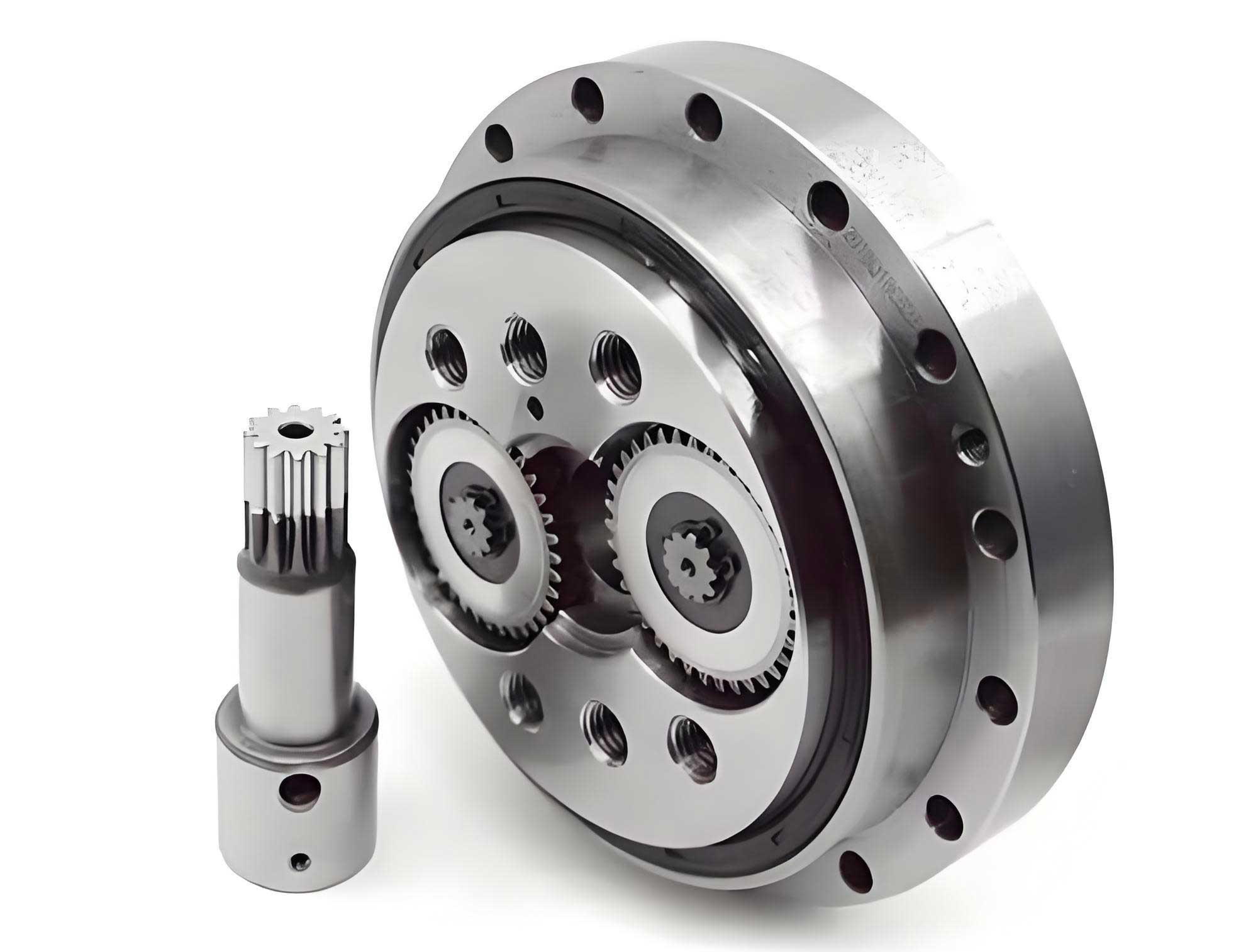
For optimization, three primary performance objectives are identified: minimizing volume, maximizing transmission efficiency, and minimizing the maximum contact stress on the cycloid gear tooth flank. These correspond directly to the desired attributes of compactness, high efficiency, and strong load-bearing capacity for the rotary vector reducer.
Volume Calculation
The overall volume of the rotary vector reducer is approximated by summing the volumes of its key rotating and structural components: the sun gear, planets, cycloid gears, pin teeth, and the针齿壳. A simplified model for volume \( V \) is given by:
$$ V = \frac{\pi}{4} m^2 b \left( Z_a^2 + 3\left( \frac{Z_a (i – 1)}{Z_p} \right)^2 \right) + \frac{\pi}{4} (D_p + D_{ap} + 2\Delta)^2 (2B + \delta) $$
where:
- \( m \): Module of the first-stage gears (mm)
- \( b \): Face width of the first-stage gears (mm)
- \( Z_a \): Number of teeth on the sun gear
- \( i \): Total transmission ratio of the rotary vector reducer
- \( Z_p \): Number of pin teeth
- \( D_p \): Pitch diameter of the pin circle (mm)
- \( D_{ap} \): Diameter of the pin (pin tooth) (mm)
- \( \Delta \): Wall thickness of the pin housing (针齿壳), typically 2 mm
- \( B \): Thickness of the cycloid gear (mm)
- \( \delta \): Gap between the two cycloid gears, typically 2.5 mm
This formulation captures the axial and radial dimensions influenced by the design variables.
Transmission Efficiency Calculation
The overall transmission efficiency \( \eta \) of the rotary vector reducer is a product of the efficiencies of its constituent stages and bearings. It can be expressed as:
$$ \eta = \left( \eta_1 \cdot \frac{\eta_2}{i} \right)^2 \times 0.992 $$
where \( 0.992 \) accounts for bearing losses (approx.). The efficiency of the cycloid stage \( \eta_1 \) and the planetary stage \( \eta_2 \) are derived from mechanical theory considering friction and multi-tooth engagement:
$$ \eta_1 = 1 – (1 – i) \left[1 – 0.0805 \left( i – 1 + \frac{Z_p}{Z_a (i – 1)} \right) \right]^3 $$
$$ \eta_2 = \frac{Z_p – 0.035(5.6 – 4.2K_1)}{Z_p + 0.035(Z_p – 1)(5.6 – 4.2K_1)} $$
Here, \( K_1 \) is the short width coefficient of the cycloid gear, a crucial design parameter affecting tooth profile and contact.
Load Capacity and Contact Stress
The maximum contact stress \( \sigma_{Hmax} \) between the cycloid gear and the pin teeth is the critical indicator for the load capacity of the rotary vector reducer. According to Hertzian contact theory, it is calculated as:
$$ \sigma_{Hmax} = 0.418 \sqrt{ \frac{F_i E_c}{B \rho_{ei}} } $$
where:
- \( F_i \): Normal load at the \(i\)-th contact point (N)
- \( E_c \): Equivalent elastic modulus (MPa), \( E_c = \frac{2E_1 E_2}{E_1 + E_2} \)
- \( B \): Cycloid gear thickness (mm)
- \( \rho_{ei} \): Equivalent radius of curvature at the contact point (mm)
The load distribution among the simultaneously engaged teeth is complex. The maximum force \( F_{max} \) on a single pin is approximated by:
$$ F_{max} = \frac{2.2 T}{K_1 Z_c R_p} $$
where \( T \) is the output torque. The force at an arbitrary meshing position \( \phi \) is \( F_i = F_{max} \frac{\sin \phi}{\sqrt{1 + K_1^2 – 2 K_1 \cos \phi}} \). To avoid iterative search for the worst-case stress, an equivalent calculation point at \( \phi = \arccos(K_1) \) is chosen, introducing an empirical coefficient \( Y_i \) (typically 1.25). The final formula for maximum equivalent contact stress becomes:
$$ \sigma_{Hmax} = 0.418 Y_i \sqrt{ \frac{F_i E_c}{B \rho_{ei}} } $$
This stress must be minimized to enhance the durability and load capacity of the rotary vector reducer.
Mathematical Model for Multi-Objective Optimization
Design Variables
Based on the analysis of the objectives, eight independent design parameters are selected as optimization variables. These parameters fundamentally define the geometry and performance of the rotary vector reducer.
$$ \mathbf{X} = [x_1, x_2, x_3, x_4, x_5, x_6, x_7, x_8]^T = [m, b, Z_a, D_p, K_1, B, Z_p, D_{ap}]^T $$
Integrated Objective Function via Weighting
The three primary objectives have different units and scales. To form a single scalar objective function, they are first normalized relative to a baseline design and then combined using weighted coefficients derived from AHP. Let \( V_0 \), \( \eta_0 \), and \( \sigma_0 \) represent the volume, efficiency, and contact stress of the initial design. A综合 performance improvement rate \( f \) is defined:
$$ f = \lambda_1 \cdot \left( \frac{V_0 – V}{V_0} \right) + \lambda_2 \cdot \left( \frac{\eta – \eta_0}{\eta_0} \right) + \lambda_3 \cdot \left( \frac{\sigma_0 – \sigma}{\sigma_0} \right) $$
where \( \lambda_1, \lambda_2, \lambda_3 \) are the weight coefficients for volume, efficiency, and contact stress, respectively, with \( \lambda_1 + \lambda_2 + \lambda_3 = 1 \). The optimization problem is then formulated as minimizing the negative of this improvement (or maximizing \( f \)):
$$ \min F(\mathbf{X}) = 1 – f(\mathbf{X}) $$
Thus, minimizing \( F(\mathbf{X}) \) directly corresponds to maximizing the weighted综合 performance improvement of the rotary vector reducer.
Constraint Conditions
The design must satisfy a series of constraints from geometric compatibility, strength criteria, and manufacturing standards. These constraints ensure the feasibility and reliability of the optimized rotary vector reducer. They are expressed as inequality constraints \( g_j(\mathbf{X}) \leq 0 \).
| Constraint Type | Mathematical Expression | Description |
|---|---|---|
| Module Limit | \( g_1(\mathbf{X}) = 1 – m \leq 0 \) | Module must be greater than 1 mm. |
| Cycloid Tooth Undercut & Pointing | \( g_2(\mathbf{X}) = r_{rp} – \frac{(1 – K_1)^2}{Z_p K_1 – 1} r_p < 0 \) | Prevents defective cycloid tooth profile. |
| Short Width Coefficient Range | \( g_3(\mathbf{X}) = K_{d1} – K_1 \leq 0 \), \( g_4(\mathbf{X}) = K_1 – K_{d2} \leq 0 \) | \( K_1 \) must lie within recommended bounds based on \( Z_c \). |
| Face Width Ratio | \( g_5(\mathbf{X}) = 5m – b \leq 0 \), \( g_6(\mathbf{X}) = b – 17m \leq 0 \) | Face width constrained relative to module. |
| Pin Tooth Spacing & Interference | \( g_7(\mathbf{X}) = 1.25(D_{ap}+2\Delta) – D_p \sin(\pi/Z_p) \leq 0 \) \( g_8(\mathbf{X}) = D_p \sin(\pi/Z_p) – 4(D_{ap}+2\Delta) \leq 0 \) |
Ensures proper pin spacing in housing. |
| Cycloid Gear Thickness | \( g_9(\mathbf{X}) = 0.05D_p – B \leq 0 \), \( g_{10}(\mathbf{X}) = B – 0.1D_p \leq 0 \) | Thickness proportional to pin circle diameter. |
| Pin Diameter Coefficient | \( g_{11}(\mathbf{X}) = 1.5 – K_2 \leq 0 \), \( g_{12}(\mathbf{X}) = K_2 – 2.0 \leq 0 \) where \( K_2 = \frac{r_p}{r_{rp}} \sin(\frac{\pi}{Z_p}) \) |
Optimal pin size relative to spacing. |
| Pin Bending Strength | \( g_{13}(\mathbf{X}) = \frac{1.41 F_{max} L}{D_{ap}^3} – \sigma_{FP} \leq 0 \) (for 2-support) or \( \frac{0.48 F_{max} L}{D_{ap}^3} – \sigma_{FP} \leq 0 \) (for 3-support) |
Pin must withstand bending stress. |
| Standard Size Range | \( g_{14}(\mathbf{X}) = D_{p1} – D_p \leq 0 \), \( g_{15}(\mathbf{X}) = D_p – D_{p2} \leq 0 \) | \( D_p \) must conform to standard model series. |
The complete optimization problem for the rotary vector reducer is:
$$ \begin{aligned}
&\min \quad F(\mathbf{X}) = 1 – f(\mathbf{X}) \\
&\text{subject to} \quad g_j(\mathbf{X}) \leq 0, \quad j = 1, 2, …, 15 \\
&\quad \mathbf{X}^L \leq \mathbf{X} \leq \mathbf{X}^U
\end{aligned} $$
where \( \mathbf{X}^L \) and \( \mathbf{X}^U \) are the lower and upper bounds of the design variables.
Determining Objective Weights Using Analytic Hierarchy Process (AHP)
The core of the proposed hierarchical optimization for the rotary vector reducer is the objective determination of the weights \( \lambda_1, \lambda_2, \lambda_3 \). AHP provides a systematic framework for this task.
Constructing the Hierarchical Model
The decision problem is decomposed into three levels:
- Goal (Level 1): Select the optimal design for the rotary vector reducer.
- Criteria (Level 2): The three optimization objectives: Volume (V), Transmission Efficiency (η), Load Capacity (represented by low Contact Stress, σ).
- Alternatives (Level 3): The various possible design parameter sets (solutions).
The focus here is on using AHP to prioritize the Criteria level with respect to the Goal.
Building the Pairwise Comparison Matrix
Experts in rotary vector reducer design are asked to compare the relative importance of each pair of criteria. The comparisons are made using a fundamental scale, translating qualitative judgments into numerical values.
| Intensity of Importance | Definition | Explanation |
|---|---|---|
| 1 | Equal Importance | Two criteria contribute equally. |
| 3 | Moderate Importance | Experience slightly favors one criterion. |
| 5 | Strong Importance | Experience strongly favors one criterion. |
| 7 | Very Strong Importance | A criterion is favored very strongly. |
| 9 | Extreme Importance | The evidence favoring one criterion is of the highest possible order. |
| 2, 4, 6, 8 | Intermediate Values | Used for compromise between adjacent judgments. |
For the three criteria (Volume, Efficiency, Contact Stress), a 3×3 pairwise comparison matrix \( \mathbf{A} \) is constructed by an expert. For instance, if Efficiency is considered moderately more important than Volume, the element \( a_{21} \) (Efficiency vs. Volume) would be 3, and its reciprocal \( a_{12} = 1/3 \). Suppose after synthesizing expert opinions, the following consistent judgment matrix is obtained for a typical rotary vector reducer application where efficiency and reliability are prioritized:
$$ \mathbf{A} = \begin{bmatrix}
1 & 1/3 & 1/2 \\
3 & 1 & 1 \\
2 & 1 & 1
\end{bmatrix} $$
Here, the rows/columns correspond to [Volume, Efficiency, Contact Stress].
Calculating Weights and Consistency Check
The weight vector \( \mathbf{W} = [\lambda_1, \lambda_2, \lambda_3]^T \) is computed using the eigenvalue method, often approximated by the geometric mean (方根法) method:
- Calculate the geometric mean of each row: \( \tilde{w}_i = \left( \prod_{j=1}^{n} a_{ij} \right)^{1/n} \).
- Normalize the geometric means to obtain the weights: \( \lambda_i = \tilde{w}_i / \sum_{k=1}^{n} \tilde{w}_k \).
For matrix \( \mathbf{A} \):
$$ \tilde{w}_1 = (1 \cdot \frac{1}{3} \cdot \frac{1}{2})^{1/3} \approx 0.550, \quad \tilde{w}_2 = (3 \cdot 1 \cdot 1)^{1/3} \approx 1.442, \quad \tilde{w}_3 = (2 \cdot 1 \cdot 1)^{1/3} \approx 1.260 $$
$$ \sum \tilde{w}_i \approx 3.252 $$
$$ \lambda_1 \approx \frac{0.550}{3.252} \approx 0.169, \quad \lambda_2 \approx \frac{1.442}{3.252} \approx 0.443, \quad \lambda_3 \approx \frac{1.260}{3.252} \approx 0.387 $$
Consistency must be verified to ensure the judgments are logically sound.
- Compute the maximum eigenvalue \( \lambda_{max} \): \( \lambda_{max} \approx \frac{1}{n} \sum_{i=1}^{n} \frac{(\mathbf{A}\mathbf{W})_i}{\lambda_i} \). For our matrix and weights, \( \lambda_{max} \approx 3.018 \).
- Calculate the Consistency Index (CI): \( CI = \frac{\lambda_{max} – n}{n – 1} = \frac{3.018 – 3}{2} = 0.009 \).
- Calculate the Consistency Ratio (CR): \( CR = \frac{CI}{RI} \), where RI is the Random Index.
| n | 1 | 2 | 3 | 4 | 5 | 6 | 7 | 8 | 9 |
|---|---|---|---|---|---|---|---|---|---|
| RI | 0 | 0 | 0.52 | 0.89 | 1.12 | 1.26 | 1.36 | 1.41 | 1.46 |
For \( n=3 \), \( RI = 0.52 \). Thus, \( CR = \frac{0.009}{0.52} \approx 0.017 \). Since \( CR < 0.10 \), the consistency of the judgment matrix is acceptable. Therefore, the weights for the rotary vector reducer optimization are taken as \( \lambda_1 \approx 0.17, \lambda_2 \approx 0.44, \lambda_3 \approx 0.39 \). This clearly shows that for this application scenario, transmission efficiency and load capacity (low stress) are significantly more important than a minimal volume reduction.
Optimization Implementation and Case Study
The integrated AHP-GA optimization framework is applied to a specific model, the RV-550E rotary vector reducer. The initial design parameters serve as the baseline for calculating the performance improvement rate \( f \).
Algorithm Flow and Setup
The optimization follows a sequential process: 1) Determine weights using AHP. 2) Use these weights to construct the weighted single-objective function \( F(\mathbf{X}) \). 3) Employ a Genetic Algorithm to solve the constrained minimization problem for \( F(\mathbf{X}) \). The GA is chosen for its ability to handle non-convex, discontinuous problems and to find a global optimum. Key GA parameters are set as follows: Population Size = 300, Maximum Generations = 100, Crossover Probability = 0.6, Mutation Probability = 0.01. Binary encoding is used for the design variables. Due to the stochastic nature of GA, the optimization is run 50 times to gather a set of potential optimal solutions.
Optimization Results and Analysis
From the 50 runs, the solution with the highest综合 performance improvement rate (lowest \( F(\mathbf{X}) \)) is selected as the optimal design. The results are summarized below, comparing the initial design with the optimized and subsequently rounded design.
| Design Variable / Performance Metric | Initial Design | Optimized Solution (GA) | Rounded & Practical Solution |
|---|---|---|---|
| Module, \( m \) (mm) | 3.0 | 1.506 | 1.5 |
| Face Width, \( b \) (mm) | 20.0 | 7.75 | 8.0 |
| Sun Gear Teeth, \( Z_a \) | 14 | 24.99 | 25 |
| Pin Circle Diameter, \( D_p \) (mm) | 330 | 349.42 | 349 |
| Short Width Coeff., \( K_1 \) | 0.80 | 0.849 | 0.85 |
| Cycloid Gear Thickness, \( B \) (mm) | 25.0 | 20.11 | 20.0 |
| Number of Pin Teeth, \( Z_p \) | 60 | 75.46 | 75 |
| Pin Diameter, \( D_{ap} \) (mm) | 10.0 | 7.63 | 8.0 |
| Volume, \( V \) (mm³) | 5.14e6 | 4.43e6 | 4.43e6 |
| Transmission Efficiency, \( \eta \)(%) | 79.9% | 82.7% | 82.7% |
| Max Contact Stress, \( \sigma_{Hmax} \) (MPa) | 878.5 | 797.43 | 797.52 |
| Overall Performance Improvement, \( f \) | 0% | 8.04% | 8.01% |
The optimization leads to significant improvements:
- Compactness: Despite an increase in \( D_p \) (radial dimension), the substantial reduction in module, face width, and cycloid gear thickness results in a net 13.8% reduction in volume, making the rotary vector reducer more compact.
- Efficiency: The increase in the number of teeth (\( Z_a \) and \( Z_p \)) improves the contact ratio in both gear stages. The transmission efficiency rises from 79.9% to 82.7%, a gain of 2.8 percentage points.
- Load Capacity: The optimized short width coefficient \( K_1 \) and other parameters reduce the maximum contact stress by 81 MPa (9.2% reduction), significantly enhancing the durability and load-bearing potential of the rotary vector reducer.
- Overall Gain: According to the AHP-weighted metric, the comprehensive performance is improved by over 8.0%, validating the effectiveness of the hierarchical multi-objective approach.
All constraint conditions are satisfied by the optimized design.
Sensitivity and Trend Analysis
Analyzing the relationship between individual design variables and the partial contributions to the综合 improvement rate reveals valuable design insights for the rotary vector reducer. For instance, the module \( m \) and face width \( b \) show a strong negative correlation with the overall performance; reducing them is highly beneficial for meeting all weighted goals. Conversely, increasing the number of teeth (\( Z_a \), \( Z_p \)) and the short width coefficient \( K_1 \) within their allowable ranges positively impacts the overall score, primarily by boosting efficiency and reducing stress. The cycloid gear thickness \( B \) exhibits a trade-off: increasing it lowers contact stress but increases volume. The optimization algorithm finds the precise balance point where the weighted sum is optimal. This sensitivity information is crucial for designers when making final adjustments to the rotary vector reducer parameters.
Conclusion
This study successfully establishes and demonstrates a robust framework for the multi-objective hierarchical optimization design of rotary vector reducers. By integrating the Analytic Hierarchy Process with a Genetic Algorithm, the method provides a systematic and rational approach to resolving the inherent trade-offs between volume, transmission efficiency, and load capacity. The AHP component quantitatively derives objective weights from expert judgment, transforming a vague multi-criteria problem into a well-defined single-objective optimization. The GA component effectively explores the complex, constrained design space to find a global optimum.
The case study on an RV-550E model confirms the practical value of this methodology. The optimized rotary vector reducer design achieves a simultaneous reduction in volume, a significant increase in transmission efficiency, and a notable decrease in critical contact stress, leading to an overall performance enhancement of 8.0%. The resulting design is not only theoretically superior but also manufacturable, as the parameters can be rounded to standard values with negligible performance loss. This AHP-GA based optimization strategy offers a powerful and generalizable tool for engineers seeking to develop high-performance, next-generation rotary vector reducers for demanding applications like precision robotics, paving the way for more efficient and reliable mechanical systems.