
In the field of advanced manufacturing, precision gear transmissions play a pivotal role, especially in applications such as industrial robots where high accuracy and reliability are paramount. The rotary vector reducer, often abbreviated as RV reducer, is a critical component in these systems due to its compact design, high torque capacity, and excellent positioning accuracy. However, the performance of a rotary vector reducer is highly sensitive to manufacturing imperfections, particularly tooth profile errors in the cycloidal gear. These errors arise during the machining process due to factors like machine tool inaccuracies, cutter wear, fixture misalignment, and gear blank variations. This article aims to delve into the impact of tooth profile errors on the transmission accuracy of the cycloidal-pin gear pair within a rotary vector reducer. Using a combination of experimental measurement data, numerical curve fitting techniques, and gear meshing theory, I will analyze how these errors alter the transmission error curve, which is a key indicator of kinematic precision. The insights gained are crucial for improving the design and manufacturing processes of high-precision rotary vector reducers used in robotics and other precision machinery.
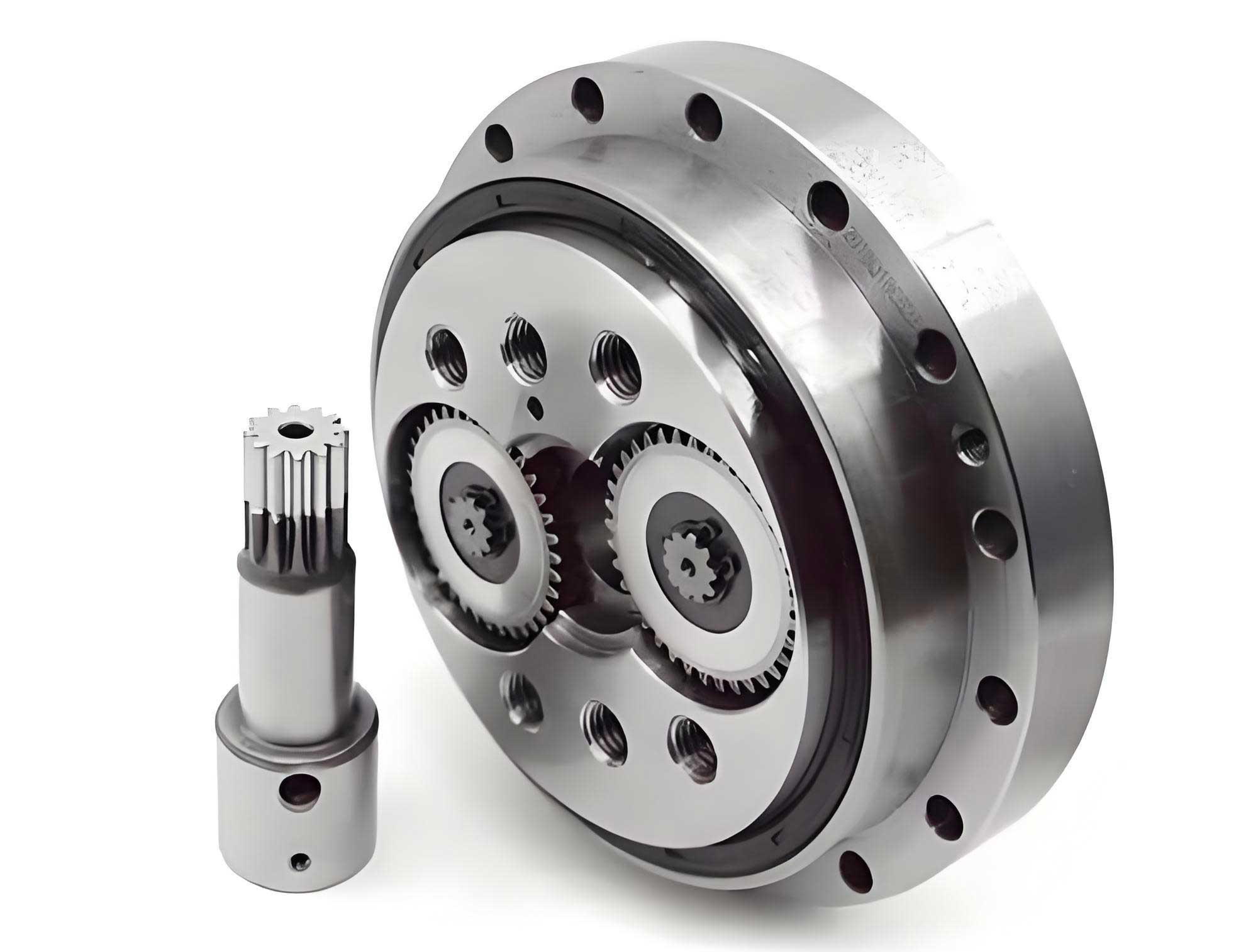
The rotary vector reducer is renowned for its two-stage reduction mechanism, typically comprising a planetary gear stage and a cycloidal-pin gear stage. The latter is responsible for the major speed reduction and high torque output. In the cycloidal stage, a cycloidal disk (or gear) meshes with a set of stationary pins arranged in a circle. The theoretical tooth profile of the cycloidal gear is derived based on epitrochoidal geometry, often modified through profile shifting and equidistant modifications to optimize contact conditions and reduce backlash. However, in practice, the manufactured tooth profile deviates from this ideal geometry due to the aforementioned errors. These tooth profile errors can lead to non-uniform load distribution, increased contact stresses, vibration, noise, and ultimately, reduced transmission accuracy and lifespan of the rotary vector reducer. Therefore, quantifying and analyzing the effect of these errors is essential for ensuring the high performance demanded by applications like robotic joints.
To begin the analysis, the first step involves obtaining the actual tooth profile data of a manufactured cycloidal gear. This is typically done using a precision gear measuring machine. In this study, a measurement setup analogous to a JD350-type cycloidal gear measuring machine is employed. The measurement points are selected at equal intervals of the meshing phase angle, ensuring a representative sampling of the entire tooth flank. Suppose we have a theoretical cycloidal gear profile given in parametric form. For a cycloidal gear with parabolic modification, the theoretical tooth profile in the transverse plane can be expressed in homogeneous coordinates as:
$$ \mathbf{r_c}(\phi) = [x_c(\phi), y_c(\phi), 0, 1]^T $$
where $\phi$ is the meshing phase angle (or generating angle), and $x_c(\phi)$ and $y_c(\phi)$ are the coordinate functions defining the ideal profile. The unit normal vector at any point on this profile is:
$$ \mathbf{n_c}(\phi) = [n_{xc}(\phi), n_{yc}(\phi), 0]^T $$
During measurement, at each specified meshing phase angle $\phi_i$ (where $i = 1, 2, 3, \dots, N$, and $N$ is the number of measurement points, e.g., 90), the deviation of the actual profile from the theoretical profile is recorded. Let $\delta’_{\phi_i}$ denote the measured profile error at point $i$, taken along the normal direction. The coordinates of the actual measured point on the tooth flank, $(X_{c_i}, Y_{c_i})$, can then be calculated as:
$$
\begin{cases}
X_{c_i} = x_c(\phi_i) + n_{xc}(\phi_i) \cdot \delta’_{\phi_i} \\
Y_{c_i} = y_c(\phi_i) + n_{yc}(\phi_i) \cdot \delta’_{\phi_i}
\end{cases}
$$
This process yields a set of discrete data points $\{ (X_{c_i}, Y_{c_i}) \}$ that represent the actual tooth surface, incorporating the tooth profile errors. The distribution of these points, based on equal meshing phase angles, ensures that regions of the tooth that are critical for load sharing and contact are adequately sampled. This discrete point cloud serves as the foundation for constructing a continuous mathematical representation of the actual tooth profile, which is necessary for subsequent contact analysis.
To perform tooth contact analysis (TCA) on a pair of gears, a continuous and differentiable representation of the tooth flanks is required. The discrete measured points must therefore be converted into a smooth curve. This is achieved using curve fitting techniques. Among various methods, Non-Uniform Rational B-Spline (NURBS) curves offer excellent flexibility and precision for representing complex shapes like gear teeth. A NURBS curve of degree $p$ is defined parametrically as:
$$ \mathbf{C}(u) = \frac{\sum_{i=0}^{n} N_{i,p}(u) w_i \mathbf{P}_i}{\sum_{i=0}^{n} N_{i,p}(u) w_i}, \quad u \in [0,1] $$
where $\mathbf{P}_i$ are the control points, $w_i$ are the weights, and $N_{i,p}(u)$ are the B-spline basis functions of degree $p$, defined recursively on a knot vector $\mathbf{U} = \{u_0, u_1, …, u_{m}\}$. For many engineering applications, cubic NURBS ($p=3$) provide a good balance between smoothness and computational efficiency. In this context, a cubic B-spline curve (a special case of NURBS with all weights equal to 1) is often sufficient for fitting gear profiles. The vector form of a cubic B-spline curve is:
$$ \mathbf{p}(u) = \sum_{i=0}^{n} \mathbf{d}_i N_{i,3}(u) $$
where $\mathbf{d}_i$ are the control point vectors, and $n+1$ is the number of control points. To fit the measured data points $\{ \mathbf{Q}_k \}$ (where $\mathbf{Q}_k = (X_{c_k}, Y_{c_k})$), a curve interpolation or approximation problem is solved. Typically, one sets up a system of equations to find the control points $\mathbf{d}_i$ such that the curve passes through or closely approximates the data points at corresponding parameter values $u_k$. The parameter values $u_k$ can be assigned using chord-length or centripetal parameterization. Once the control points are determined, the NURBS curve $\mathbf{R}_c(u) = [x(u), y(u)]$ provides a digital tooth profile that incorporates the measured tooth profile errors. This digital profile is continuously differentiable, allowing for the calculation of tangents and normals needed for contact analysis.
It is crucial to verify the accuracy of the NURBS fitting. Since the fitted curve is a constructed approximation, its deviation from the actual measured points (or from the theoretical curve if fitting error-free data) must be assessed. A validation procedure can be implemented as follows: First, take a set of points from the theoretical tooth profile at the same meshing phase angles used for measurement. Fit a NURBS curve to these theoretical points. Then, select a different set of points at distinct meshing phase angles (e.g., 37 points) on the theoretical profile. Compute the normal distance between these new theoretical points and the corresponding points on the fitted NURBS curve. The maximum normal deviation should be negligibly small (e.g., on the order of $10^{-8}$ mm) to confirm that the fitting error is insignificant compared to the magnitude of the tooth profile errors. This ensures that the NURBS representation faithfully captures the geometric features and can reliably replace the actual tooth profile in subsequent simulations.
With the digital tooth profile of the cycloidal gear established, the next step is to perform tooth contact analysis (TCA) for the cycloidal-pin gear pair, considering the influence of tooth profile errors. TCA is a computational method used to determine the kinematic transmission error, contact patterns, and bearing contact under loaded or unloaded conditions. For the rotary vector reducer’s cycloidal stage, we consider the engagement between the cycloidal gear and the fixed pin wheel. A coordinate system must be defined to describe the relative motion. Let $S_c$ be a coordinate system rigidly attached to the cycloidal gear, and $S_p$ be a coordinate system attached to the pin wheel (or to an individual pin, but typically the pins are fixed in the housing). The fixed global frame is denoted $S_f$. The cycloidal gear rotates about its axis with an angle $\phi_2$, while the pin wheel is considered stationary (or its rotation $\phi_1$ is considered for kinematic analysis, but in the RV reducer, the pin wheel is fixed, and the output is from the cycloidal gear via a carrier; however, for transmission error calculation, relative motion is key).
The surface of the cycloidal gear in $S_c$ is given by the fitted NURBS curve $\mathbf{R}_c(u) = [x_c(u), y_c(u), 0]^T$. The surface of a pin (assumed cylindrical) in $S_p$ can be represented as:
$$ \mathbf{R}_p(\beta, l) = [r_{rp} \cos\beta, -r_{rp} \sin\beta, l]^T $$
where $r_{rp}$ is the pin radius, $\beta$ is an angular parameter around the pin circumference, and $l$ is the length coordinate (though for 2D analysis in the transverse plane, $l$ is ignored). However, for TCA, we often consider the center of the pin. The pin center relative to the pin wheel coordinate system is at a fixed radius $r_p$ (the distribution circle radius). Through coordinate transformations, both surfaces are expressed in the fixed coordinate system $S_f$. The condition for contact between the cycloidal gear tooth and a pin is that at the contact point, the position vectors and the surface normals coincide (assuming continuous tangency). This leads to a set of equations known as the meshing equations. For a given rotation angle $\phi_1$ of the pin wheel (or equivalently, the input angle), we solve for the parameter $u$ on the cycloidal tooth, the angle $\beta$ on the pin, and the rotation angle $\phi_2$ of the cycloidal gear such that:
$$ \mathbf{r}_f^{(c)}(u, \phi_2) = \mathbf{r}_f^{(p)}(\beta, \phi_1) $$
$$ \mathbf{n}_f^{(c)}(u, \phi_2) = \mathbf{n}_f^{(p)}(\beta, \phi_1) $$
where $\mathbf{r}_f^{(c)}$ and $\mathbf{r}_f^{(p)}$ are the position vectors of points on the cycloidal tooth and pin surface, respectively, expressed in $S_f$, and $\mathbf{n}_f^{(c)}$ and $\mathbf{n}_f^{(p)}$ are the corresponding unit normals. In practice, since the pins are circular and fixed, the problem can be simplified. The condition often reduces to finding the point on the cycloidal tooth profile that is at a distance equal to the pin radius from the pin center, with the cycloidal tooth normal passing through the pin center. For each angular position of the cycloidal gear (or pin wheel), the contact point is determined. By varying the input angle $\phi_1$ incrementally, a series of contact points are obtained, representing the path of contact.
The transmission error (TE) is defined as the deviation of the actual output position from the theoretically ideal output position, given a uniform input motion. For a gear pair with gear ratio $i = z_p / z_c$, where $z_p$ is the number of pins and $z_c$ is the number of cycloidal teeth, the theoretical output rotation for an input rotation $\phi_1$ is $\phi_{2,ideal} = (z_p / z_c) \phi_1$. The actual output rotation $\phi_2$ is determined from the TCA solution. The transmission error $\Delta E$ is then:
$$ \Delta E(\phi_1) = \phi_2(\phi_1) – \phi_{20} – \frac{z_p}{z_c} (\phi_1 – \phi_{10}) $$
where $\phi_{10}$ and $\phi_{20}$ are reference angles at a chosen initial contact point (often where the transmission error is defined as zero). Transmission error is usually expressed in arc minutes or arc seconds for precision gears like those in a rotary vector reducer. The curve of $\Delta E$ versus $\phi_1$ over one mesh cycle reveals the kinematic accuracy. In an ideal gear pair without errors, the transmission error curve would be a straight horizontal line at zero (or a constant). However, due to manufacturing errors and intentional modifications, it typically exhibits periodic variations.
To illustrate the methodology, let’s consider a specific example of a rotary vector reducer’s cycloidal-pin gear pair. The basic geometric parameters are summarized in the table below.
| Parameter Name | Symbol | Value |
|---|---|---|
| Number of cycloidal teeth | $z_c$ | 11 |
| Number of pins | $z_p$ | 12 |
| Pin radius | $r_{rp}$ | 7 mm |
| Eccentricity | $a$ | 4 mm |
| Pin distribution circle radius | $r_p$ | 90 mm |
| Equidistant modification amount | $\Delta r_{rp}$ | 0.01 mm |
| Profile shift modification amount | $\Delta r_p$ | -0.02 mm |
The theoretical tooth profile of the cycloidal gear with these modifications can be derived. For brevity, the detailed equations are omitted, but they follow standard epitrochoidal geometry with corrections. Now, suppose the tooth profile errors are measured on an actual manufactured cycloidal gear. The measured profile errors (in micrometers) at 90 points along one tooth flank are tabulated. For the sake of this example, let’s assume the error values follow a pattern similar to typical manufacturing variations. A subset of these errors is presented in the following table to illustrate the data structure.
| Point Index | Error (μm) | Point Index | Error (μm) | Point Index | Error (μm) | Point Index | Error (μm) |
|---|---|---|---|---|---|---|---|
| 1 | 0.1 | 24 | 4.0 | 48 | -0.9 | 72 | 2.4 |
| 2 | 0.3 | 25 | 2.9 | 49 | 0.2 | 73 | 2.7 |
| 3 | 0.7 | 26 | 2.6 | 50 | -0.1 | 74 | 2.8 |
| 4 | 1.7 | 27 | 2.7 | 51 | 0.1 | 75 | 3.3 |
| 5 | 2.7 | 28 | 1.8 | 52 | 0.3 | 76 | 3.8 |
| 6 | 3.7 | 29 | 1.6 | 53 | 0.5 | 77 | 3.6 |
| 7 | 4.8 | 30 | 1.0 | 54 | 0.7 | 78 | 3.4 |
| 8 | 5.8 | 31 | 1.3 | 55 | 1.2 | 79 | 3.2 |
| 9 | 6.6 | 32 | 0.9 | 56 | 1.4 | 80 | 2.7 |
| 10 | 6.8 | 34 | 0.5 | 57 | 1.5 | 81 | 3.1 |
| 11 | 7.2 | 35 | 0.1 | 58 | 1.7 | 82 | 3.8 |
| 12 | 7.7 | 36 | -0.2 | 59 | 1.9 | 83 | 3.4 |
| 13 | 8.3 | 37 | -0.1 | 60 | 2.1 | 84 | 2.5 |
| 14 | 5.8 | 38 | -0.7 | 61 | 3.2 | 85 | 1.7 |
| 15 | 8.2 | 39 | -0.5 | 62 | 3.6 | 86 | 1.8 |
| 16 | 8.2 | 40 | -0.1 | 63 | 3.9 | 87 | 1.2 |
| 17 | 7.2 | 41 | -0.3 | 64 | 4.3 | 88 | 0.5 |
| 18 | 7.2 | 42 | -0.6 | 65 | 3.5 | 89 | 0.1 |
| 19 | 7.6 | 43 | -0.7 | 66 | 3.3 | 90 | -0.1 |
| 20 | 6.7 | 44 | -0.8 | 67 | 3.4 | ||
| 21 | 5.7 | 45 | -0.5 | 68 | 3.2 | ||
| 22 | 4.8 | 46 | -0.2 | 69 | 3.2 | ||
| 23 | 4.6 | 47 | -0.4 | 70 | 2.6 |
Using these error values, the actual coordinate points are computed via the earlier formula. Then, a cubic NURBS curve is fitted to these points. The control points are calculated, and the curve is obtained. The fitted digital tooth profile is denoted $\mathbf{R}_c(u)$. As part of the validation, the fitting error is checked by comparing the fitted curve to the theoretical profile at points not used in fitting. The maximum normal deviation is found to be on the order of $1 \times 10^{-8}$ mm, which is negligible, confirming the accuracy of the NURBS representation.
Now, with the digital tooth profile that includes tooth profile errors, the tooth contact analysis is performed. A computer program implementing the TCA algorithm is developed. For each incremental angle of the input (which, in the context of a rotary vector reducer, can be considered as the rotation of the crankshaft or the wave generator that excites the cycloidal gear’s eccentric motion), the contact point between the cycloidal tooth and a specific pin is determined by solving the meshing equations numerically. This yields the corresponding output angle $\phi_2$. The transmission error $\Delta E$ is then computed according to the formula above. The process is repeated for a full cycle of engagement, typically corresponding to one tooth mesh (i.e., as the cycloidal gear rotates through an angle of $360^\circ / z_c$ relative to the pins).
The results are plotted to compare the transmission error curves. First, consider the theoretical case with no tooth profile errors. In this ideal scenario, the transmission error curve, when plotted against input angle (or normalized mesh phase), appears as a smooth parabolic-like shape due to the intentional profile modifications (equidistant and shift modifications). This curve typically has a single peak and is relatively flat near the peak, indicating a well-designed modification that aims to minimize transmission error variation and ensure smooth motion transfer. For the given parameters, the theoretical transmission error curve might look like a downward-opening parabola with a maximum amplitude of a few arc seconds or minutes, depending on the modification amounts.
Next, we examine the transmission error curve when tooth profile errors are considered. Using the fitted digital tooth profile from the measured error data, the TCA yields a different curve. The presence of tooth profile errors introduces additional irregularities into the gear mesh. The resulting transmission error curve is no longer a smooth parabola. Instead, it exhibits a wavy pattern with multiple peaks and valleys. Specifically, for the error data given, the curve might show two distinct peaks within one mesh cycle, and these peaks are sharper (steeper) compared to the theoretical curve. Moreover, the amplitude of the transmission error (i.e., the peak-to-peak variation) is generally larger than in the theoretical case. The crossing points of the curve (where it passes through zero) may not be symmetrically placed. These observations indicate that tooth profile errors significantly alter both the shape and the magnitude of the transmission error.
To quantify the impact, we can define some metrics. Let $TE_{max}$ be the maximum positive deviation, $TE_{min}$ the minimum negative deviation, and $TE_{pp} = TE_{max} – TE_{min}$ the peak-to-peak transmission error. For the theoretical curve, these values might be, for example, $TE_{max, theory} = 1.2$ arc minutes, $TE_{min, theory} = -0.8$ arc minutes, giving $TE_{pp, theory} = 2.0$ arc minutes. For the curve with errors, the values could be $TE_{max, error} = 2.5$ arc minutes, $TE_{min, error} = -1.5$ arc minutes, resulting in $TE_{pp, error} = 4.0$ arc minutes. This demonstrates a doubling of the peak-to-peak transmission error due to the introduced tooth profile errors. Such an increase can be detrimental for the precision of a rotary vector reducer, as these reducers are often required to have transmission errors less than 1 arc minute and backlash under tight tolerances for robotic applications.
The waviness in the transmission error curve is directly correlated with the spatial frequency of the tooth profile errors. Since the errors were measured at discrete points and likely contain both low-frequency (form error) and high-frequency (roughness) components, the fitted NURBS curve smooths out some high-frequency content but retains the overall form error. The resulting transmission error curve reflects this, showing oscillations that correspond to the error pattern along the tooth flank. This underscores the importance of controlling tooth profile errors during manufacturing to achieve the desired kinematic performance in a rotary vector reducer.
Beyond the kinematic transmission error, tooth profile errors also affect other aspects of gear performance, such as load distribution and contact stress. While this analysis focuses on unloaded TCA (kinematic error), the same digital tooth profile can be used in loaded tooth contact analysis (LTCA) to study these effects. In LTCA, the elastic deformations of the teeth and supporting structures are considered, and the contact pattern and stress distribution are computed under load. The presence of profile errors can lead to edge loading, stress concentrations, and uneven load sharing among multiple teeth in contact, which is critical for the durability of the rotary vector reducer. Therefore, the methodology presented here serves as a foundation for more comprehensive mechanical analysis.
In summary, this article has presented a detailed methodology for analyzing the influence of tooth profile errors on the transmission error of the cycloidal-pin gear pair in a rotary vector reducer. The approach combines experimental measurement, NURBS curve fitting, and numerical tooth contact analysis. The key steps are: (1) Measure the tooth profile errors at discrete points along the tooth flank using a gear measuring machine. (2) Compute the actual surface coordinates by superimposing the errors onto the theoretical profile along the normal direction. (3) Fit a NURBS curve (e.g., cubic B-spline) to the measured points to obtain a continuous digital tooth profile. (4) Perform TCA by solving the meshing equations for the digital cycloidal tooth and the ideal pins. (5) Compute the transmission error curve and compare it with the theoretical error-free case.
The example analysis clearly shows that tooth profile errors can substantially change both the shape and amplitude of the transmission error curve. The theoretical smooth parabolic curve transforms into a wavy curve with increased peak-to-peak variation. This degradation in kinematic accuracy can compromise the performance of the rotary vector reducer in precision applications. Hence, manufacturers should strive to minimize tooth profile errors through careful control of machining processes, tooling, and quality inspection. Additionally, the digital tooth profile model developed here can be integrated into broader simulation frameworks for dynamic analysis, fatigue life prediction, and optimization of the rotary vector reducer design.
Future work could extend this analysis to include other manufacturing errors such as pitch errors, runout, and assembly errors (e.g., eccentricity errors, bearing clearances). Moreover, the interaction between multiple cycloidal teeth in simultaneous contact could be studied using loaded contact analysis. The effect of lubrication and thermal effects might also be considered. Nevertheless, the current study provides a robust and practical method for assessing the impact of tooth profile errors on the transmission accuracy of cycloidal gears in rotary vector reducers, contributing to the advancement of high-precision gear technology for robotics and other demanding fields.
To reiterate, the rotary vector reducer is a cornerstone of modern robotic drive systems, and its transmission precision is critical. By understanding and mitigating the effects of tooth profile errors through advanced analysis techniques like the one described, engineers can design and produce more reliable and accurate reducers. This, in turn, enhances the performance of industrial robots, enabling finer motions, higher repeatability, and longer service life. The continuous pursuit of such improvements is essential as the demand for advanced automation grows across various sectors, from manufacturing to healthcare.