
The precision and reliability of modern industrial robots are fundamentally dependent on the performance of their core transmission components. Among these, the Rotary Vector (RV) reducer stands as one of the two most prevalent types of reducers used in robotic joints, alongside harmonic drives. The distinctive advantages of the RV reducer, including its compact size, high torque density, substantial reduction ratio, excellent torsional stiffness, and minimal backlash, make it indispensable for applications demanding high precision and repeatability. As the manufacturing and adoption of RV reducers have progressed into commercial-scale production, the imperative for comprehensive and accurate performance evaluation has grown significantly. This necessitates the development of specialized testing systems capable of quantifying both static and dynamic parameters. While dynamic performance, such as transmission efficiency and fatigue life, is crucial, the foundational characteristics are defined by its static performance parameters. These parameters, including torsional stiffness, backlash (lost motion), transmission accuracy, and hysteresis, directly influence the positioning accuracy, rigidity, and responsiveness of the robotic system. Presently, a standardized, integrated system for evaluating all key static performance metrics of RV reducers remains an area requiring focused development. This article details the research and development of such a holistic static testing system, exploring the theoretical basis, design methodology, and experimental implementation for characterizing the static behavior of RV reducers.
Static Performance Parameters of RV Reducers
The static performance of an RV reducer is typically characterized under loaded but non-rotating (or quasi-static) conditions. The relationship between the applied input torque and the resulting angular displacement at the output, when measured through a full loading and unloading cycle, yields a hysteresis characteristic curve. This closed-loop curve encapsulates all major static performance metrics. The primary parameters derived from this curve are defined below.
1. Torsional Stiffness (KT): This is the most critical indicator of an RV reducer’s resistance to elastic deformation under load. It is defined as the ratio of the applied torque to the resulting torsional angular deflection within the linear elastic region of the reducer’s operation. A higher torsional stiffness signifies less angular displacement for a given torque, leading to better positional accuracy and dynamic response of the robot arm. It is calculated from the linear portion of the hysteresis curve’s slope.
$$K_T = \frac{\Delta T}{\Delta \theta}$$
where $\Delta T$ is the change in torque and $\Delta \theta$ is the corresponding change in angular displacement (often in radians or arc-minutes). Units are typically N·m/rad or N·m/arcmin.
2. Backlash or Lost Motion (L): This parameter quantifies the inherent mechanical clearance or “play” within the RV reducer, primarily stemming from gear tooth flank clearances and bearing fits. It manifests as a dead zone where input rotation does not produce output movement when the direction of rotation is reversed. On the hysteresis curve, it is represented by the width of the loop at zero torque. It is formally measured at a low torque level (e.g., ±2% or ±3% of the rated torque).
$$L = |\theta_{T=+T_s}| + |\theta_{T=-T_s}|$$
where $T_s$ is a small threshold torque (e.g., 3% of rated torque) and $\theta$ is the angular position at that torque during loading/unloading.
3. Transmission Accuracy (or Positioning Error, E): This defines the RV reducer’s ability to achieve a precise output angle for a given input command under load. It is the maximum deviation between the actual output angle and the theoretically expected output angle (considering the ideal reduction ratio) when the reducer is loaded to its rated torque. On the hysteresis curve, it is often taken as the total angular displacement at the rated torque point.
$$E = \theta_{T=T_{rated}}$$
It is a comprehensive error including the effects of elastic deformation and non-linearities.
4. Hysteresis (H): The area enclosed by the loading and unloading curves represents the energy loss per cycle due to internal friction, micro-slip in contacts, and material damping. While not always a separately reported parameter, it is a valuable indicator of the RV reducer’s mechanical efficiency and repeatability in static or low-speed conditions.
The relationship between these parameters and the hysteresis curve is summarized in the following conceptual diagram and table.
| Parameter | Symbol | Definition | Typical Unit | Source on Hysteresis Curve |
|---|---|---|---|---|
| Torsional Stiffness | $K_T$ | Slope of the linear torque-angle region | N·m/rad, N·m/arcmin | Inverse slope of linear fitting |
| Backlash (Lost Motion) | $L$ | Angular displacement at near-zero torque during direction reversal | arcmin, mrad | Width of loop at $T ≈ 0$ |
| Transmission Accuracy | $E$ | Total angular deviation at rated torque | arcmin, mrad | $\theta$ value at $T = T_{rated}$ |
| Hysteresis | $H$ | Area enclosed by the loading/unloading loop | J/cycle | Area of the closed curve |
Theoretical Foundation and Finite Element Analysis of RV Reducer Stiffness
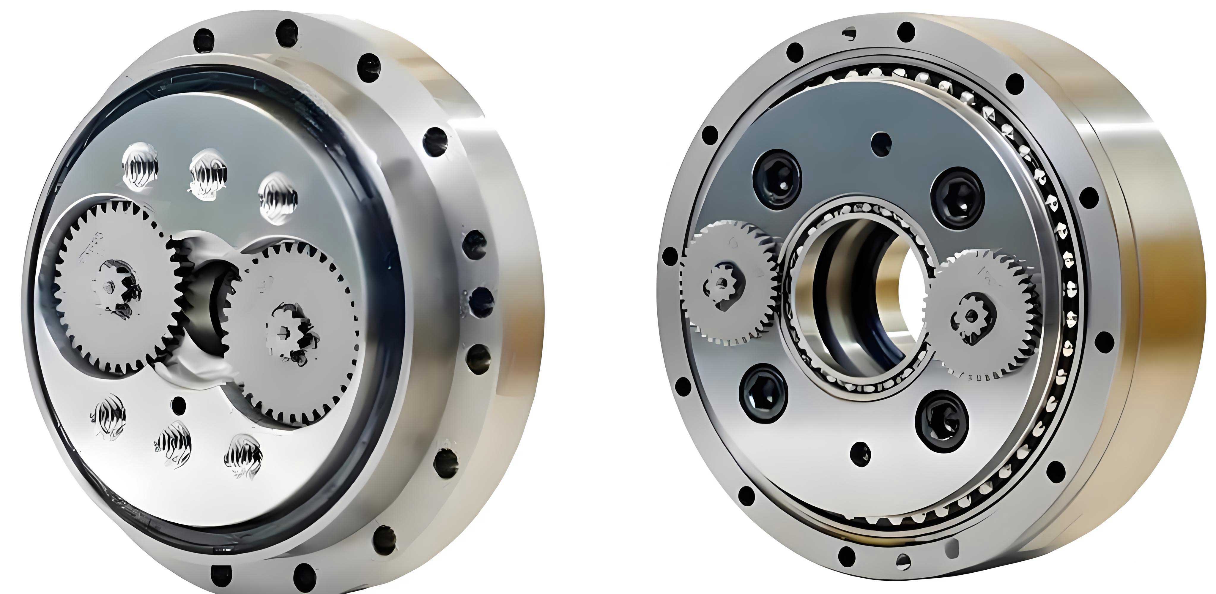
The unique structure of the RV reducer, combining a first-stage planetary gear train with a second-stage cycloidal pinwheel mechanism, gives it exceptional stiffness. The torsional stiffness is not a simple constant but is influenced by design parameters such as gear tooth profiles, bearing stiffness, and particularly the geometry of the cycloidal disc. A key parameter affecting the latter is the eccentricity ($a$) of the crankshaft. The relationship between eccentricity and stiffness can be explored through theoretical modeling and Finite Element Analysis (FEA).
In a simplified theoretical model, the deformation of the cycloidal disc under load is a major contributor to the overall compliance of the RV reducer. The torsional stiffness can be approximated by considering the bending and contact deformation of the cycloidal disc lobes. An increase in eccentricity generally leads to a larger force transmission angle and altered contact conditions within the cycloid-pin engagement, typically resulting in increased system stiffness.
To validate this relationship and understand the stress distribution, a static structural simulation was conducted using ANSYS Workbench. A simplified 3D model of an RV reducer assembly was created, focusing on the critical load-bearing components: the input gear, crankshafts, cycloidal discs, pins, and the output housing. The model was assigned appropriate material properties (e.g., alloy steel for gears and bearings). A fixed support was applied to the output flange, while a gradually increasing torque was applied to the input shaft. The primary output was the angular deflection of the input relative to the fixed output.
The FEA results clearly demonstrated the trend. For an RV reducer model under a constant input torque, the total angular deformation decreased as the crankshaft eccentricity was increased. The following table summarizes the findings from the simulation, and the governing equation for stiffness calculation is shown.
The torsional stiffness $K_T$ is calculated from the FEA results as:
$$K_T = \frac{T_{applied}}{\theta_{max}}$$
where $\theta_{max}$ is the maximum angular deformation obtained from the simulation.
| Crankshaft Eccentricity, $a$ (mm) | Applied Input Torque, $T$ (N·m) | Maximum Angular Deformation, $\theta_{max}$ (arcmin) | Calculated Torsional Stiffness, $K_T$ (N·m/arcmin) | Trend |
|---|---|---|---|---|
| 1.2 | 1000 | 3.85 | 259.7 | Baseline |
| 1.3 | 1000 | 3.52 | 284.1 | Increase |
| 1.4 | 1000 | 3.25 | 307.7 | Increase |
The simulation confirms that increasing the eccentricity parameter $a$ reduces the elastic angular deformation for a given load, thereby increasing the overall torsional stiffness of the RV reducer. This insight is crucial for both the design optimization of new RV reducers and for understanding the performance variations between different models. The FEA serves as a vital virtual prototyping tool before physical testing.
Architecture of the Integrated Static Testing System
The core objective of this development project was to create a unified, automated, and accurate platform capable of generating the complete hysteresis curve for an RV reducer and extracting all static performance parameters in a single, controlled test sequence. The system is designed around a PC-based control architecture and integrates three fundamental modules: the Torque Loading Module, the Sensing and Detection Module, and the Data Acquisition and Control Module.
1. Torque Loading Module
This module is responsible for applying a precisely controlled rotational force to the RV reducer’s input shaft and providing a controlled, variable load at its output shaft. It consists of:
- Servo Drive System: A high-precision AC servo motor and its matching digital servo driver. This system provides the input rotation. Its speed and position are controlled with high resolution to execute the slow, quasi-static test profile.
- Motion Control Card: Installed in the industrial PC, this card receives high-level commands from the testing software and generates the precise pulse trains required to control the servo driver, managing the motion trajectory (speed, direction, acceleration).
- Load Simulation Unit: A magnetorheological (MR) brake or a precision magnetic powder brake is attached to the output flange of the RV reducer. This device acts as the variable load. Its output braking torque is linearly proportional to its excitation current, allowing for computer-controlled, stepless torque application via a programmable current controller.
2. Sensing and Detection Module
This module measures the two critical physical quantities: torque and angular displacement.
- Torque Measurement: Two high-accuracy, non-contact rotary torque sensors are employed. One is placed between the servo motor and the RV reducer input to measure the actual input torque ($T_{in}$). A second sensor can be placed after the RV reducer output to measure the output torque ($T_{out}$) for potential efficiency calculations, though for pure static hysteresis, the input sensor is primary. These sensors typically utilize strain gauges with wireless or slip-ring signal transmission to ensure noise-free data.
- Angular Displacement Measurement: An ultra-high-resolution rotary optical encoder (or “ring encoder”) is mounted directly on the output shaft of the RV reducer. This device measures the absolute or incremental angular position of the output with arc-second or better resolution, which is essential for accurately capturing the minute deformations of the RV reducer.
3. Data Acquisition and Control Module
This is the “brain” of the system, coordinating all actions and collecting all data.
- Industrial Computer (IPC): Hosts the custom testing software, data processing algorithms, and user interface.
- Data Acquisition (DAQ) Card: Captures analog voltage signals from the torque sensors and digital pulse signals from the optical encoder with synchronized timing.
- Software Platform: Developed in a platform like LabVIEW or with C++/Python using relevant libraries. It performs:
- Test sequence automation (control of servo motion and brake current).
- Real-time data acquisition and visualization.
- Post-processing of the hysteresis data (curve fitting, parameter calculation).
- Data logging and report generation.
| Module | Key Components | Primary Function |
|---|---|---|
| Torque Loading | Servo Motor & Driver, Motion Control Card, Magnetic Brake, Current Controller | Apply controlled input motion and variable output load. |
| Sensing & Detection | Input/Output Torque Sensors, High-Resolution Optical Encoder | Measure input torque and output angular displacement with high precision. |
| Data Acquisition & Control | Industrial PC, DAQ Card, Custom Testing Software | Automate test sequence, acquire synchronized data, process results. |
Experimental Procedure and Data Analysis Workflow
The testing procedure is a fully automated cycle designed to trace the upper and lower branches of the hysteresis curve. The following steps outline a complete test for an RV reducer with a rated torque $T_R$.
Step 1: System Initialization and Test Preparation
The RV reducer is securely mounted in the test fixture. The motion control axes and DAQ channels are initialized. The maximum test torque is set, typically to 150-200% of the rated torque ($T_{max} = 1.5T_R$ to $2T_R$) to ensure the linear region is fully characterized. The corresponding excitation current for the magnetic brake is calculated from its torque-current characteristic and pre-set in the current controller. The servo motor is enabled.
Step 2: Forward Loading Phase
The servo motor begins a very slow clockwise rotation. The magnetic brake provides a resisting torque, loading the RV reducer. The DAQ system continuously records the increasing input torque $T(t)$ from the torque sensor and the corresponding accumulated angular displacement $\theta(t)$ from the optical encoder on the output. This continues until $T(t)$ reaches the predetermined positive maximum torque $+T_{max}$. At this point, the forward loading curve (from origin to point A) is recorded.
Step 3: Forward Unloading and Reverse Loading Phase
The servo motor reverses direction (counter-clockwise). The torque begins to decrease from $+T_{max}$, moving along the upper hysteresis branch. The angular displacement $\theta(t)$ decreases. When the torque passes through zero, the angular displacement may not be zero due to backlash, creating the curve’s width. The motor continues, now applying torque in the negative direction. The torque value becomes increasingly negative until it reaches the negative maximum torque $-T_{max}$. This phase traces the curve from point A through the upper zero-torque crossing to point B.
Step 4: Reverse Unloading Phase
The servo motor reverses direction again (back to clockwise). The torque increases from $-T_{max}$ towards zero, tracing the lower hysteresis branch. The angular displacement increases from its most negative value back towards zero. The phase ends when the torque returns approximately to zero, completing the hysteresis loop from point B back to the origin (or a point near it, indicating residual deformation).
Step 5: System Shutdown
The servo motor stops. The excitation current to the magnetic brake is ramped down to zero. The motion control and DAQ systems are safely disabled. The raw time-series data of $T(t)$ and $\theta(t)$ is saved.
Data Processing and Parameter Extraction:
The raw data pairs $(T_i, \theta_i)$ are plotted to form the hysteresis loop. Sophisticated algorithms in the testing software then analyze this curve:
- Linear Region Identification: The software identifies the most linear segments of the loading and unloading branches, typically excluding the initial low-torque non-linear zone (backlash zone) and any region near the maximum torque if saturation occurs.
- Stiffness Calculation: A linear regression (least-squares fit) is performed on the selected linear region data points. The torsional stiffness $K_T$ is the inverse of the slope $m$ of this fitted line.
$$K_T = \frac{1}{m}, \quad \text{where } m = \frac{\Delta \theta}{\Delta T} \text{ from linear fit}$$ - Backlash Calculation: The software finds the angular displacement values at a small threshold torque (e.g., $T_s = \pm0.03T_R$) on both the loading and unloading branches. The total backlash $L$ is the sum of the absolute values of these two angles.
$$L = |\theta(T=+T_s)| + |\theta(T=-T_s)|$$ - Transmission Accuracy Calculation: The total angular displacement at the rated torque $\theta(T_R)$ is read directly from the forward loading curve. This value represents the transmission error under full load.
$$E \approx \theta(T=T_R)$$
| Phase | Servo Motor Action | Torque State | Data Acquisition | Curve Segment Traced |
|---|---|---|---|---|
| 1. Preparation | Enable, Hold | $T=0$ | Begin | Origin |
| 2. Forward Loading | Slow CW Rotation | $0 \rightarrow +T_{max}$ | Continuous | Lower-to-Upper Branch (0→A) |
| 3. Fwd Unload / Rev Load | Slow CCW Rotation | $+T_{max} \rightarrow -T_{max}$ | Continuous | Upper Branch (A→B via zero) |
| 4. Reverse Unloading | Slow CW Rotation | $-T_{max} \rightarrow 0$ | Continuous | Lower Branch (B→0) |
| 5. Shutdown | Stop | Hold at 0 | Stop & Save | Hysteresis Loop Complete |
Conclusion and Future Perspectives
The development of a dedicated, integrated static testing system for RV reducers marks a significant step towards the rigorous characterization and quality assurance of these critical robotic components. By automating the acquisition of the hysteresis characteristic curve, this system provides a reliable, repeatable, and efficient method for quantifying the fundamental static performance parameters: torsional stiffness, backlash, and transmission accuracy. The integration of Finite Element Analysis during the design phase allows for valuable insights into the influence of geometric parameters like eccentricity on stiffness, bridging the gap between theoretical design and empirical performance. The modular architecture of the system, comprising precise torque loading, high-fidelity sensing, and automated data acquisition/control, ensures that the testing process is both comprehensive and adaptable to different RV reducer models and specifications.
The implications of this work are multifold. For RV reducer manufacturers, such a system provides an essential tool for quality control in mass production, enabling batch testing and performance grading. For research and development teams, it serves as a critical platform for validating new designs, materials, or lubrication strategies aimed at enhancing performance—for instance, developing an RV reducer with higher stiffness or lower backlash. Furthermore, by establishing a standardized testing methodology, it allows for objective performance comparison between different RV reducer products, fostering healthy competition and technological advancement in the industry. Future enhancements to this testing system could involve the integration of thermal chambers to study performance under varying temperature conditions, the addition of vibration analysis sensors for more comprehensive dynamic-static coupling studies, and the implementation of machine learning algorithms for predictive maintenance and anomaly detection based on the hysteresis curve morphology. Ultimately, the continued refinement of testing technologies for critical components like the RV reducer is foundational to achieving the next levels of precision, reliability, and intelligence in industrial automation and robotics.