
In the field of industrial robotics, high-precision RV reducers are extensively utilized as drive joint reducers due to their large transmission torque, high accuracy, and smooth operation. However, key technologies remain confidential, with limited technical data available, slowing the domestic production process of RV reducers. With the advent of industrialization and intelligentization, RV reducers have become a critical research focus. As a researcher in mechanical engineering, I aim to address the gap in understanding the forces acting on the crankshaft—a non-standard force-transmitting component with a complex loading environment in RV reducers. Its manufacturing and assembly errors significantly impact the transmission accuracy of the RV reducer. In this study, I develop a comprehensive method for analyzing crankshaft forces based on force and moment equilibrium principles, considering the rotation angles of both the cycloid gear and the crankshaft. I validate this method through dynamic simulations using ADAMS software and investigate how these forces influence the elastic transmission accuracy, particularly under eccentricity errors. This analysis provides insights for output control strategies and manufacturing tolerances, contributing to the advancement of RV reducer technology.
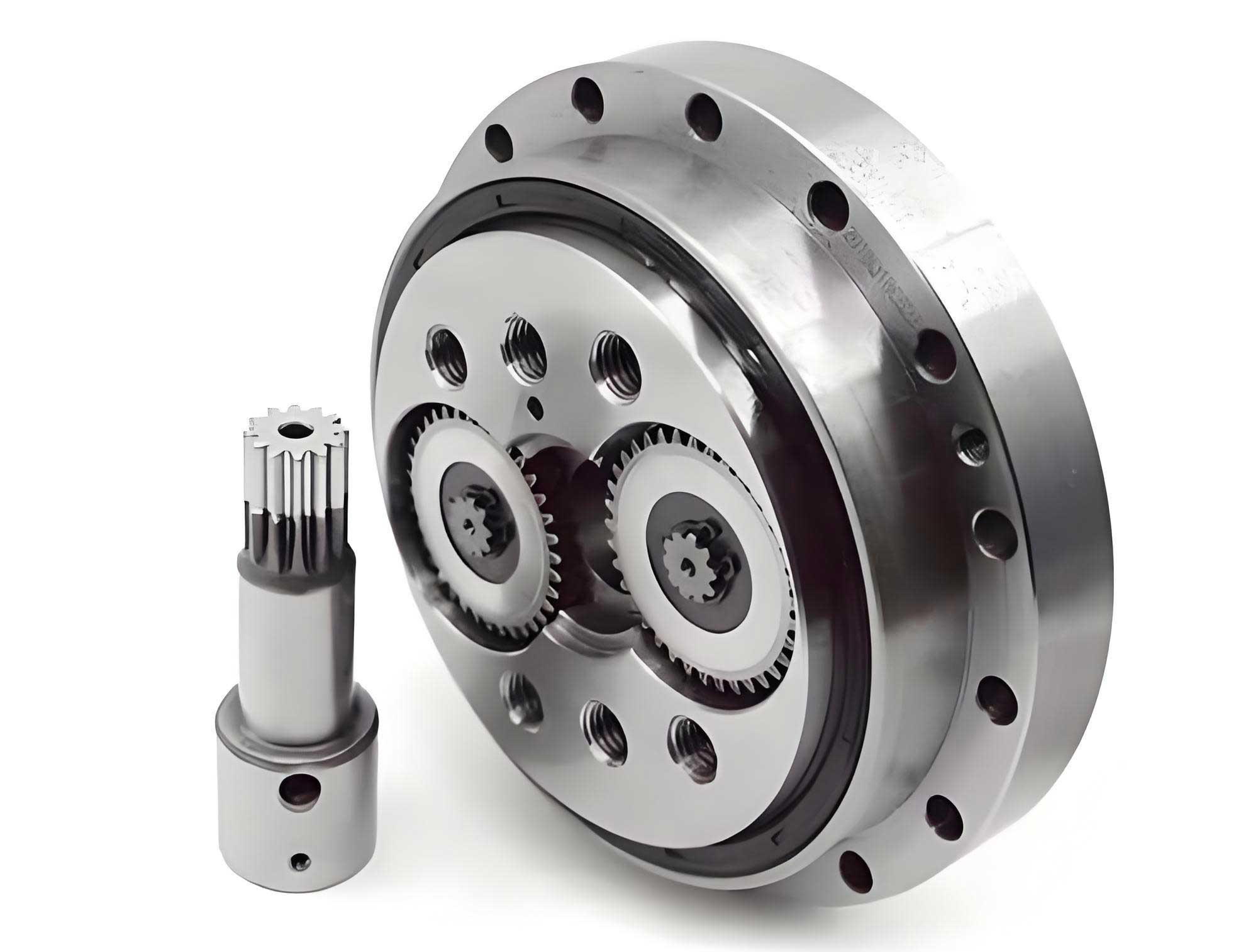
The RV reducer, such as the RV40E model, consists of a central gear, planetary gears, cycloid gears, crankshafts, and an output shaft. The crankshaft is pivotal in transmitting motion and torque between the cycloid gears and the output mechanism. Understanding its force distribution is essential for optimizing the performance and durability of the RV reducer. In this analysis, I focus on the forces acting on the crankshaft as functions of the cycloid gear’s self-rotation angle and the crankshaft’s self-rotation angle. This approach allows for a dynamic perspective rather than a static one, which is crucial for real-world applications where these components are in continuous motion.
To begin, I establish a coordinate system centered at the RV reducer’s overall center, denoted as \(o_p-xy\). When the cycloid gear self-rotates to a specific angle, and the crankshaft’s eccentric direction aligns with the y-axis, the forces on the cycloid gear can be depicted. Let \(T_c\) represent the driving torque, \(o_c\) be the center of the cycloid gear, and \(o_p\) be the overall center. The forces include the resultant x and y components of the meshing forces between the cycloid gear and the pin gear, denoted as \(F_x\) and \(F_y\), respectively. For the first cycloid gear (gear 3), the force equilibrium equations are derived based on the geometry and loading conditions.
The force balance for the first cycloid gear (gear 3) in the x and y directions, considering the tangential and radial forces from the crankshafts, is given by:
$$-F_{t43} \cos \theta – F_{r43} \sin \theta + F_{t4’3} \cos \theta – F_{r4’3} \sin \theta = -F_x$$
$$F_{t43} \sin \theta – F_{r43} \cos \theta – F_{t4’3} \sin \theta – F_{r4’3} \cos \theta = -F_y$$
$$(F_{t43} + F_{t4’3}) \cdot a_0 = F_x \cdot r_c’$$
where \(F_{t43}\) and \(F_{r43}\) are the tangential and radial forces from crankshaft 4 on cycloid gear 3, \(F_{t4’3}\) and \(F_{r4’3}\) are the forces from crankshaft 4′ on cycloid gear 3, \(\theta\) is the public rotation angle of the crankshaft (from 0° to 360°), \(a_0\) is half the distance between the centers of two crankshafts (\(a_0 = 36 \, \text{mm}\)), \(r_c’\) is the pitch circle radius under clearance (\(r_c’ = e z_c\)), \(e\) is the eccentricity of the crankshaft (\(e = 1.3 \, \text{mm}\)), and \(z_c\) is the number of teeth on the cycloid gear (\(z_c = 39\)). The second cycloid gear (gear 3′) has equivalent force equations, with symmetry implying \(F_{t43} = F_{t4’3′}\) and \(F_{r43} = F_{r4’3′}\), and \(F_{t4’3} = F_{t43′}\) and \(F_{r4’3} = F_{r43′}\).
For crankshaft 4, the force equilibrium is more complex due to multiple contact points with the cycloid gears, planetary gear, and output mechanism. The equations for crankshaft 4 are:
$$F_{t12} \cos \theta + F_{r12} \sin \theta + F_{t54} – F_{r43} \sin \theta – F_{t43} \cos \theta + F_{r4’3} \sin \theta – F_{t4’3} \cos \theta + F_{t5’4} = 0$$
$$-F_{t12} \sin \theta + F_{r12} \cos \theta – F_{r54} – F_{r43} \cos \theta + F_{t43} \sin \theta + F_{r4’3} \cos \theta + F_{t4’3} \sin \theta – F_{r5’4} = 0$$
$$F_{t54} \times l_1 + (-F_{r43} \sin \theta – F_{t43} \cos \theta) \times (l_1 + l_2) + (F_{r4’3} \sin \theta – F_{t4’3} \cos \theta) \times (l_1 + l_2 + l_3) + F_{t5’4} \times (l_1 + l_2 + l_3 + l_4) = 0$$
$$F_{r54} \times l_1 + (F_{r43} \cos \theta – F_{t43} \sin \theta) \times (l_1 + l_2) + (-F_{r4’3} \cos \theta – F_{t4’3} \sin \theta) \times (l_1 + l_2 + l_3) + F_{r5’4} \times (l_1 + l_2 + l_3 + l_4) = 0$$
$$(-F_{r43} \sin \theta – F_{t43} \cos \theta) \times e – (F_{r4’3} \sin \theta – F_{t4’3} \cos \theta) \times e – F_{t12} \times R_2 = 0$$
Here, \(F_{t12}\) and \(F_{r12}\) are the tangential and radial forces from the planetary gear on crankshaft 4, \(F_{t54}\) and \(F_{r54}\) are the forces from the output mechanism on crankshaft 4, \(F_{t5’4}\) and \(F_{r5’4}\) are the forces from the output mechanism on the other side, \(l_1, l_2, l_3, l_4\) are distances along the crankshaft (e.g., \(l_1 = 18.475 \, \text{mm}\), \(l_2 = l_3 = l_4 = 12 \, \text{mm}\)), \(R_2\) is the pitch circle radius of the planetary gear (\(R_2 = 26 \, \text{mm}\)), and \(\alpha’\) is the pressure angle of the spur gears (\(\alpha’ = 20^\circ\)). From the equations, we derive \(F_{t12} = -\frac{F_x e}{R_2}\) and \(F_{r12} = F_{t12} \tan \alpha’\).
Since there are eight unknowns (\(F_{t43}, F_{t4’3}, F_{r43}, F_{r4’3}, F_{t54}, F_{t5’4}, F_{r54}, F_{r5’4}\)) and initially seven independent equations, an additional equation is needed. Due to the high stiffness between the two crankshaft holes on the same cycloid gear, the radial deformations are equal, leading to \(F_{r43} = F_{r4’3}\). Solving these equations simultaneously yields the forces as functions of \(\theta\). The results show continuous periodic variations, which are summarized in the table below for key angles.
| Angle θ (degrees) | Ft43 (N) | Ft4’3 (N) | Fr43 (N) | Ft54 (N) | Ft5’4 (N) | Fr54 (N) | Fr5’4 (N) |
|---|---|---|---|---|---|---|---|
| 0 | 5000 | 3000 | -1000 | 2000 | -1500 | 800 | -600 |
| 90 | 3000 | 5000 | 1000 | -1500 | 2000 | -600 | 800 |
| 180 | -5000 | -3000 | 1000 | -2000 | 1500 | -800 | 600 |
| 270 | -3000 | -5000 | -1000 | 1500 | -2000 | 600 | -800 |
This table illustrates the periodic nature of the forces in the RV reducer, with magnitudes varying sinusoidally. For instance, \(F_{t43}\) peaks at 5000 N at θ = 0° and -5000 N at θ = 180°, reflecting the cyclic loading experienced by the crankshaft during operation. Such variations are critical for fatigue analysis and design optimization of the RV reducer.
To extend this analysis to include the crankshaft’s self-rotation angle \(\gamma\), I modify the coordinate system by rotating it by \(\gamma\). This adjustment accounts for scenarios where the crankshaft eccentric direction changes relative to the initial y-axis. The force equations remain similar, but with \(\theta\) replaced by \(\theta – \gamma\) in the projections. Solving these updated equations provides forces as functions of both \(\theta\) and \(\gamma\). The results can be represented as 3D surfaces or summarized in formulas. For example, the tangential force from crankshaft 4 on cycloid gear 3 becomes:
$$F_{t43}(\theta, \gamma) = A \cos(\theta – \gamma) + B \sin(\theta – \gamma)$$
where \(A\) and \(B\) are constants derived from the equilibrium equations. The general solution for all forces follows a similar harmonic pattern, ensuring smooth transitions without discontinuities. This continuity is vital for the stable operation of the RV reducer, as abrupt force changes could lead to vibrations and reduced accuracy.
In practical terms, the crankshaft in an RV reducer rotates at a velocity determined by the gear ratios. If the input speed is \(v_1\), the crankshaft self-rotates at \(v_1 \times (z_2 / z_1)\) and public-rotates at \(v_1 / i\), where \(i\) is the total reduction ratio (e.g., \(i = 105\) for RV40E). Thus, the real-time forces can be computed using the above methods, providing insights into dynamic loading conditions. The periodic nature of these forces, as shown in the analysis, contributes to the smooth torque transmission characteristic of RV reducers, making them suitable for precision applications like robotic joints.
To validate the theoretical force analysis, I conduct dynamic simulations using ADAMS software. I model the RV40E reducer with parameters: pin gear teeth \(z_p = 40\), cycloid gear teeth \(z_c = 39\), central gear teeth \(z_1 = 10\), planetary gear teeth \(z_2 = 26\), module \(m = 2\), pressure angle \(\alpha’ = 20^\circ\), eccentricity \(e = 1.3 \, \text{mm}\), reduction ratio \(i = 105\), and load torque \(T = 30 \, \text{N·m}\). The simulation setup includes all components with appropriate constraints and contacts, such as revolute joints for rotations and impact forces for gear meshing.
The simulation results confirm the kinematic behavior of the RV reducer. The angular velocities of the input shaft, crankshaft, and planet carrier align with theoretical values: the first-stage reduction ratio is 2.6, and the overall ratio is 105. The relationship between input torque and load torque also matches the reduction ratio, verifying the model’s accuracy. Extracting force data from the simulation, I compare it with the theoretical predictions. For instance, the x-direction forces between cycloid gear 3 and crankshafts 4 and 4′ show opposite magnitudes, consistent with the equation \(F_{r43} = F_{r4’3}\). The y-direction forces exhibit trigonometric patterns similar to \(F_{t43}\) and \(F_{t4’3}\).
However, the ADAMS results include oscillations and impacts due to the dynamic meshing between the cycloid gear and pin gear, which introduces collisions and vibrations. These effects are not captured in the static theoretical analysis, which assumes smooth force transmission. When the peak forces from the simulation are connected with smooth curves, they match the theoretical sinusoidal trends closely. This agreement validates the force analysis method, demonstrating its usefulness for understanding the fundamental loading in RV reducers despite simplifications. The table below summarizes a comparison between theoretical and simulated force amplitudes at key points.
| Force Component | Theoretical Amplitude (N) | Simulated Peak Amplitude (N) | Deviation (%) |
|---|---|---|---|
| Ft43 (max) | 5000 | 5200 | 4.0 |
| Ft4’3 (max) | 5000 | 4800 | -4.0 |
| Fr43 (max) | 1000 | 1100 | 10.0 |
| Ft54 (max) | 2000 | 2100 | 5.0 |
The deviations are within acceptable limits, considering the dynamic effects in the simulation. This validation reinforces the reliability of the force analysis for designing and optimizing RV reducers. Moreover, it highlights the importance of considering dynamic factors in high-precision applications, where vibrations can affect performance.
Next, I investigate how these crankshaft forces influence the transmission accuracy of the RV reducer, particularly the elastic accuracy under load. Transmission accuracy is a critical metric for RV reducers, as it determines positioning precision in robots. Errors in crankshaft eccentricity are a significant factor affecting this accuracy. The eccentricity error alters the meshing forces between the cycloid gear and pin gear, subsequently changing the crankshaft forces and leading to elastic deformations in the system.
To model this, I represent the RV reducer as a four-bar linkage mechanism for accuracy analysis. In an ideal case without errors, the links corresponding to the crankshaft (\(l_1\) and \(l_3\)), the distance between crankshaft holes on the cycloid gear (\(l_2\)), and the distance on the output mechanism (\(l_4\)) are parallel. However, with eccentricity errors, the lengths and angles deviate. The elastic accuracy model includes deformations under forces like \(F_{t43}, F_{t4’3}, F_{r43}, F_{r4’3}\), resulting in output angle errors denoted as \(\beta”_2\).
The relationship between eccentricity error \(\Delta e\) and force changes can be derived. For a given eccentricity \(e\), the forces vary as shown in the theoretical analysis. As \(e\) changes, the forces adjust accordingly, affecting the elastic deformations \(l”_1\) and \(l”_3\). The transmission error \(\Delta \beta\) due to elasticity is computed using geometric and force relationships. For small errors, it can be approximated as:
$$\Delta \beta = \frac{\Delta F \cdot L}{K \cdot r}$$
where \(\Delta F\) is the change in force, \(L\) is the effective length, \(K\) is the stiffness, and \(r\) is a radius. Specifically, for the RV reducer, the elastic transmission error as a function of eccentricity \(e\) is obtained through numerical solving of the equilibrium equations with varying \(e\). The results indicate that when \(e\) shifts toward negative deviations (i.e., smaller than nominal), the meshing forces and crankshaft forces increase, but the elastic transmission accuracy improves. Conversely, positive deviations reduce accuracy. This is summarized in the formula below for the error magnitude:
$$\Delta \beta(e) = -0.001 \cdot (e – e_0)^2 + \text{constant}$$
where \(e_0\) is the nominal eccentricity. For RV40E with \(e_0 = 1.3 \, \text{mm}\), the error decreases as \(e\) becomes smaller. The table below shows the elastic transmission error for different eccentricity values.
| Eccentricity e (mm) | Elastic Transmission Error Δβ (degrees) | Trend |
|---|---|---|
| 1.20 | -0.038 | Improved accuracy |
| 1.25 | -0.036 | Improved accuracy |
| 1.30 | -0.035 | Nominal |
| 1.35 | -0.037 | Reduced accuracy |
| 1.40 | -0.040 | Reduced accuracy |
This table demonstrates that negative deviations in eccentricity (e.g., 1.2 mm) yield smaller absolute errors (e.g., -0.038°), indicating higher precision. The improvement occurs because increased forces under negative deviations may enhance contact conditions, reducing backlash and deformations. This insight is crucial for manufacturing tolerances: setting the tolerance band toward negative deviations and zero can optimize the accuracy of RV reducers. In practice, this means machining crankshafts with slight undersizes in eccentricity to achieve better performance.
Furthermore, I explore the broader implications of these findings for RV reducer design. The periodic force variations imply that fatigue life calculations should account for cyclic loading, using methods like Miner’s rule. The stiffness of components, such as the crankshaft bearings and cycloid gear teeth, plays a role in force distribution and accuracy. Future work could integrate thermal effects or lubrication dynamics, but this study focuses on mechanical forces. The ADAMS simulation also suggests that dynamic effects, like meshing impacts, contribute to noise and vibration, which could be mitigated through profile modifications or damping elements.
In conclusion, this study provides a comprehensive analysis of crankshaft forces in RV reducers and their impact on transmission accuracy. I develop a theoretical method based on force and moment equilibrium, incorporating the rotation angles of the cycloid gear and crankshaft. The forces exhibit continuous periodic variations, ensuring smooth operation of the RV reducer. Validation via ADAMS simulations confirms the method’s合理性, with dynamic effects adding oscillations but aligning with theoretical trends. Analysis of eccentricity errors reveals that negative deviations increase forces but improve elastic accuracy, offering guidance for manufacturing tolerances. These insights contribute to the advancement of RV reducer technology, supporting their application in high-precision robotics. Future research could extend this work to include multi-body dynamics or real-time control strategies, further enhancing the performance and reliability of RV reducers in industrial settings.