
In the field of industrial robotics, precision motion control is paramount. The RV reducer, or Rotary Vector reducer, serves as a critical core component in robotic joints, responsible for providing high torque, high reduction ratios, and exceptional positional accuracy with minimal backlash. As a sophisticated, integrated mechanical system comprising a primary planetary gear stage and a secondary cycloidal pin-wheel stage, the RV reducer inevitably generates vibrations during operation. These vibrations are not merely byproducts; they are rich sources of information reflecting the internal dynamic interactions, health status, and overall performance of the reducer. Excessive or abnormal vibration directly impacts the positioning accuracy of robotic arms, induces chatter, accelerates component wear, and ultimately affects the reliability and lifespan of the entire robotic system. Therefore, a deep and systematic investigation into the vibration characteristics of the RV reducer is fundamental for performance optimization, condition monitoring, and predictive maintenance.
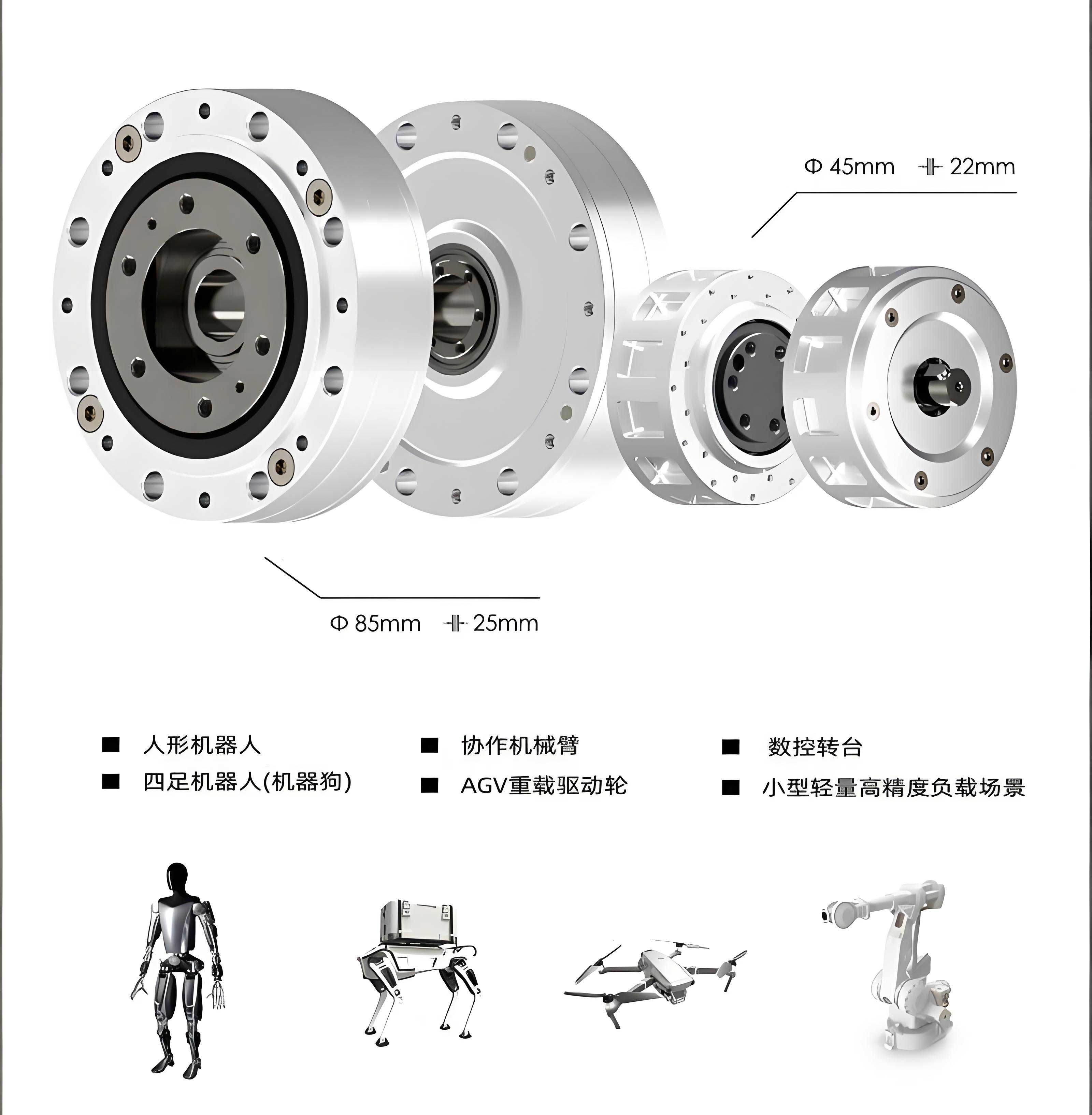
The vibrational behavior of an RV reducer is a complex phenomenon resulting from multiple excitation sources. These include time-varying meshing stiffness from both the planetary and cycloidal gear pairs, manufacturing errors such as eccentricity and profile deviations, assembly clearances, and varying load conditions. Unlike simple gearboxes, the RV reducer’s unique structure with eccentric shafts and rolling elements introduces specific periodic excitations. While theoretical modeling and simulation, such as lumped-parameter torsional models or finite element analysis, provide valuable insights into natural frequencies and mode shapes, they often rely on assumptions that may not capture all real-world complexities. Consequently, experimental vibration testing and signal analysis are indispensable for validating theories, understanding actual dynamic responses, and establishing baselines for healthy operation. Our study focuses on the comprehensive experimental vibration analysis of a domestic SHPŔ-20E type RV reducer, employing a multi-faceted signal processing approach to unravel its vibrational signature under various operating conditions.
Theoretical Foundations of Vibration Signal Processing
The vibration signal acquired from an RV reducer is typically a one-dimensional time series, $x(t)$, representing acceleration, velocity, or displacement over time. Analyzing this signal requires tools from both the time and frequency domains to extract meaningful features.
Time-Domain Analysis
Time-domain analysis examines the signal’s amplitude variation directly with time. Statistical parameters offer a concise numerical description. For a discrete vibration signal sequence ${x_i}$ with $N$ samples, key parameters include:
- Mean Value: $\mu_x = \frac{1}{N}\sum_{i=1}^{N} x_i$. For vibration signals, this often approximates zero.
- Root Mean Square (RMS): $X_{RMS} = \sqrt{\frac{1}{N}\sum_{i=1}^{N} x_i^2}$. This is a crucial measure of the overall vibration energy or intensity.
- Peak-to-Peak Value: $X_{pp} = \max(x_i) – \min(x_i)$.
- Standard Deviation: $\sigma_x = \sqrt{\frac{1}{N-1}\sum_{i=1}^{N} (x_i – \mu_x)^2}$, representing the dispersion of the signal.
- Skewness and Kurtosis: These higher-order statistics describe the asymmetry and “peakedness” of the signal’s probability distribution, sensitive to impulsive features.
Another powerful time-domain concept is the characterization of signal complexity using fractal dimension, such as the correlation dimension $D_2$. For a reconstructed phase space trajectory from the time series, $D_2$ is estimated by examining the scaling of the correlation sum $C(r)$:
$$C(r) = \lim_{N \to \infty} \frac{2}{N(N-1)} \sum_{i=1}^{N} \sum_{j=i+1}^{N} H(r – ||\mathbf{Y}_i – \mathbf{Y}_j||)$$
where $H$ is the Heaviside step function, $\mathbf{Y}_i$ are phase space vectors, and $r$ is a distance scale. The correlation dimension is given by:
$$D_2 = \lim_{r \to 0} \frac{\log C(r)}{\log r}$$
Vibration signals from a system in a stable operating state tend to exhibit a consistent fractal dimension, while changes due to developing faults can alter this measure, providing a sensitive diagnostic indicator.
Frequency-Domain Analysis
Frequency-domain analysis transforms the time signal to reveal its constituent frequency components. The primary tool is the Fast Fourier Transform (FFT), an efficient algorithm for computing the Discrete Fourier Transform (DFT):
$$X(k) = \sum_{n=0}^{N-1} x(n) e^{-j 2\pi k n / N}, \quad k = 0, 1, …, N-1$$
The power spectral density (PSD), $S_{xx}(f) = \lim_{T \to \infty} \frac{1}{T} |X(f)|^2$, shows how signal power is distributed across frequencies, identifying dominant meshing frequencies, bearing frequencies, and their harmonics, which are characteristic of the RV reducer’s kinematics.
For complex signals where periodic components are masked by sidebands or noise, cepstrum analysis is highly effective. The power cepstrum is defined as the inverse Fourier transform of the logarithm of the power spectrum:
$$C_p(\tau) = \mathcal{F}^{-1} \{ \log S_{xx}(f) \}$$
This process, often called “spectrum of a spectrum,” simplifies the detection of harmonic families and periodic structures in the spectrum, making it easier to identify the “quefrency” $\tau$ (analogous to time) corresponding to the period of spectral ripples, which often relates to fault periods.
Time-Frequency Analysis: The Wavelet Transform
Vibration signals from RV reducers under varying loads or during transients are non-stationary. The Wavelet Transform provides a time-frequency representation. The Continuous Wavelet Transform (CWT) of a signal $x(t)$ is:
$$WT(a, b) = \frac{1}{\sqrt{|a|}} \int_{-\infty}^{\infty} x(t) \, \psi^*\left(\frac{t-b}{a}\right) dt$$
where $\psi(t)$ is the mother wavelet, $a$ is the scale parameter (inversely related to frequency), and $b$ is the translation parameter (related to time). For practical discrete analysis, the Discrete Wavelet Transform (DWT) uses orthogonal filter banks to decompose a signal into approximation (low-frequency) and detail (high-frequency) coefficients at multiple resolution levels. This multi-resolution analysis (MRA) capability allows for isolating transient events and analyzing signal features at specific scales of interest, which is invaluable for fault diagnosis in the complex vibration environment of an RV reducer.
Experimental Methodology and Setup
To conduct a thorough vibration analysis, a dedicated test rig and precise measurement system were utilized. The core of the experiment was a domestic SHPŔ-20E type RV reducer mounted on a comprehensive performance test bench. This bench allowed for precise control of the input speed via a servo motor and application of controlled output torque loads.
The vibration measurement system was designed for high fidelity and isolation from electrical noise. Key components included:
- Accelerometers: High-sensitivity, capacitive MEMS-type uniaxial accelerometers (model analogous to 1C102) were employed. Their key specifications are summarized in Table 1.
- Data Acquisition System: A high-performance, multi-channel dynamic signal analyzer (analogous to DH8305) was used. Its high input isolation (>120 dB CMRR) ensured that the measured signals from the RV reducer were free from contamination by drive motor or other electromagnetic interference, guaranteeing accuracy.
- Software: Advanced signal processing software was used for real-time data acquisition, recording, and subsequent in-depth analysis.
| Parameter | Value / Description |
|---|---|
| Sensitivity | Approx. 20 mV/(m/s²) |
| Measurement Range | ±100 m/s² |
| Frequency Range | 0 – 1000 Hz |
| Resonant Frequency | > 2.7 kHz |
| Mounting Method | Adhesive bonding |
Considering the compact structure and limited external surface area of the RV reducer, three measurement points were strategically placed on its housing to capture the three-dimensional vibration response, as illustrated in the following textual description. These points were aligned to measure vibrations primarily along the three orthogonal axes of the reducer’s coordinate frame.
- Point 1 (Axis-X): Positioned to capture vibrations predominantly in the axial direction of the input/output shafts.
- Point 2 (Axis-Z): Positioned to capture vibrations in the vertical direction relative to the reducer’s mounting.
- Point 3 (Axis-Y): Positioned to capture vibrations in the horizontal direction, perpendicular to the shaft axis.
The test matrix was designed to investigate the influence of two critical operational parameters: speed and load. Tests were conducted under two main schemes:
1. Constant Speed, Variable Load: The input speed was held constant at 500 rpm, and the output load was varied through several steps.
2. Constant Load (No-load), Variable Speed: The RV reducer was run under no external load, and the input speed was varied incrementally from a low range to a high range (e.g., 200 to 2000 rpm).
For all tests, the data acquisition sampling frequency was set at 5000 Hz, sufficiently high to avoid aliasing for the frequency components of interest in an RV reducer.
Time-Domain Vibration Analysis
The raw time-domain signals offer an immediate, intuitive view of the RV reducer’s dynamic behavior. Under a baseline condition of 500 rpm input speed and moderate load, the waveform characteristics were distinctly different across the three measurement points.
A prominent visual feature in the signals from Point 1 (axial) and Point 3 (horizontal) was the presence of a “beat” pattern or amplitude modulation. Critically, the number of these beats per revolution of the output shaft corresponded directly to the number of eccentric shafts within the RV reducer. The SHPŔ-20E model incorporates three eccentric shafts, and precisely three beats were observed per output shaft cycle. This is a fundamental signature of the cycloidal stage’s kinematics, where the eccentric motion of the three shafts generates a three-peak-per-revolution forcing function. In contrast, the signal from Point 2 (vertical) was of significantly lower amplitude, appearing almost as low-level noise, indicating that the dominant vibration energy was not directed in this axis for this particular mounting configuration.
The statistical parameters calculated from these time series provide a quantitative foundation. Table 2 presents these values for the baseline test condition.
| Parameter | Point 1 (Axial, X) | Point 2 (Vertical, Z) | Point 3 (Horizontal, Y) |
|---|---|---|---|
| Maximum (m/s²) | 0.310 | 0.012 | 0.103 |
| Minimum (m/s²) | -0.325 | -0.012 | -0.119 |
| Mean (m/s²) | ~0.002 | ~ -0.001 | ~ -0.004 |
| Standard Deviation, $\sigma$ (m/s²) | 0.062 | 0.003 | 0.022 |
| Root Mean Square, RMS (m/s²) | 0.062 | 0.003 | 0.022 |
| Peak-to-Peak (m/s²) | 0.635 | 0.023 | 0.223 |
The RMS value is the most common metric for overall vibration severity. The maximum RMS value of 0.062 m/s² was observed at Point 1 (axial). Comparing this to established benchmarks for premium RV reducers (where acceptable vibration acceleration is often below 0.1 m/s² under normal operation), the tested unit’s vibration level falls within a normal, healthy range.
Influence of Operational Parameters
The effect of load and speed on the RV reducer’s vibration was systematically quantified. Figure 5 (conceptual) shows the trend of vibration RMS for Points 1 and 3 increasing with applied torque at a constant 500 rpm speed, while Point 2’s vibration remained negligible. This increase is attributed to higher mesh forces and bearing reaction forces under load. Table 3 provides sample data from this load variation test.
| Load Condition | Point 1 (X) RMS | Point 2 (Z) RMS | Point 3 (Y) RMS |
|---|---|---|---|
| Low Load (20% Tn) | 0.045 | 0.0028 | 0.015 |
| Medium Load (50% Tn) | 0.056 | 0.0029 | 0.020 |
| Rated Load (100% Tn) | 0.078 | 0.0031 | 0.028 |
Similarly, under no-load conditions, increasing the input speed led to a rise in vibration RMS for Points 1 and 3. This is expected as the frequency and magnitude of dynamic excitations (e.g., meshing impacts, unbalance forces) generally increase with speed. The data trend is summarized in Table 4.
| Input Speed (rpm) | Point 1 (X) RMS | Point 2 (Z) RMS | Point 3 (Y) RMS |
|---|---|---|---|
| 200 | 0.008 | 0.0005 | 0.003 |
| 1000 | 0.085 | 0.0040 | 0.030 |
| 1800 | 0.152 | 0.0045 | 0.055 |
Frequency-Domain Vibration Analysis
Transforming the time-domain signals to the frequency domain reveals the spectral composition of the vibration, linking specific frequency components to physical phenomena within the RV reducer.
Spectral Analysis (FFT)
The Power Spectral Density (PSD) plots for Points 1 and 3 under the 500 rpm condition revealed a highly consistent and dominant feature: a sharp peak at 186.6 Hz. The amplitude at this frequency was significantly higher than at other frequencies. For Point 1, the amplitude was approximately 0.0146 m/s², and for Point 3, it was 0.0058 m/s². This frequency is a key characteristic frequency of the RV reducer and can be related to its kinematical parameters. For instance, with an input speed of 500 rpm (8.333 Hz) and a known reduction ratio $i$, certain mesh frequencies or their harmonics will manifest. The precise identification of this 186.6 Hz peak requires knowledge of the gear teeth counts and structure but confirms the presence of a strong, synchronous excitation source. The spectrum for Point 2 showed no dominant peaks, with all amplitudes below 0.001 m/s², consistent with its low energy level.
Cepstrum Analysis
Cepstrum analysis was applied to the power spectra of the high-vibration signals (Points 1 and 3) to detect any families of harmonics or periodic structures that might be less obvious in the standard spectrum. The cepstrum transforms harmonic spacing in the spectrum into distinct peaks in the “quefrency” domain.
The results indicated that the real cepstrum showed some periodicity related to the fundamental excitation. However, the complex cepstrum and, more notably, the inverse complex cepstrum processed with a rectangular window function yielded more pronounced and isolated features. Peaks in the inverse complex cepstrum effectively highlighted the periodic components within the vibration signal’s spectral structure. This demonstrates that cepstral analysis, particularly using the inverse complex cepstrum, is a powerful tool for deconvolving the source of vibrations in a complex system like an RV reducer, potentially separating transmission path effects from the source characteristics.
Wavelet Transform Analysis
To analyze the non-stationary characteristics and transient events at multiple resolutions, Discrete Wavelet Transform (DWT) was performed on the axial and horizontal vibration signals. The Haar wavelet, due to its simplicity and effectiveness in detecting abrupt changes, was chosen for this multi-level decomposition.
The signal was decomposed into approximation coefficients (A) representing the low-frequency trend and detail coefficients (D) representing high-frequency details at each level. The process can be represented as a filter bank operation. At the first decomposition level, the original signal $S$ is split:
$$S = A1 + D1$$
Subsequent levels decompose the approximation further:
$$A1 = A2 + D2, \quad A2 = A3 + D3, \quad …$$
Our analysis showed that by the 5th level of decomposition ($D5$), the detail coefficients began to clearly exhibit a periodic pattern that correlated with the three-beat-per-revolution phenomenon observed in the time domain. While the early-level detail coefficients (D1, D2) contained mostly high-frequency noise and very fine transients, the lower-frequency oscillations associated with the eccentric shaft rotation became isolated and visible in the later detail levels (D4, D5). This multi-resolution capability is a significant advantage. It allows for the selective filtering of signal components: high-level approximations capture very low-frequency drift, mid-level details capture the main fault-related modulations (like our three-beat pattern), and low-level details capture high-frequency impacts or noise. This separation is invaluable for diagnosing specific faults in an RV reducer, such as distinguishing a bearing defect (high-frequency bursts in D1/D2) from an eccentricity-related issue (modulation in D4/D5). The mathematical representation of the decomposition down to level 5 is:
$$S = A5 + D5 + D4 + D3 + D2 + D1$$
where the characteristic periodic fault signature was most discernible in the $D5$ component for this particular signal.
Synthesis of Findings and Discussion
The comprehensive experimental analysis of the SHPŔ-20E RV reducer yields a coherent picture of its vibration characteristics. The dominant vibration energy is channeled along the axial (X) and horizontal (Y) axes of the reducer housing, with minimal energy in the vertical (Z) axis under the tested mounting configuration. This directional preference is likely influenced by the stiffness anisotropy of the housing and the primary direction of forces from the cycloidal disc meshing and bearing reactions.
The three-beat-per-revolution pattern in the time domain is a fundamental fingerprint of this RV reducer’s three-eccentric-shaft design. Any deviation from this clear, regular pattern in future tests could indicate issues like uneven load sharing among the cycloidal pins, eccentric shaft bearing wear, or misalignment.
The strong spectral peak at 186.6 Hz under the 500 rpm operating condition is a critical signature. This frequency can be tracked as a function of input speed ($f_{in}$) to confirm its origin. If it scales linearly with $f_{in}$ (e.g., $f_{peak} = k \cdot f_{in}$), it is likely a shaft rotational harmonic or a fixed meshing order component. Identifying this relationship is key for establishing a health baseline; the appearance of new spectral peaks or sidebands around this fundamental frequency in a used RV reducer would be a strong indicator of developing faults like tooth pitting or localized bearing defects.
The utility of advanced signal processing techniques is clearly demonstrated. While RMS values from the time domain are excellent for overall severity monitoring, they lack diagnostic specificity. Spectral (FFT) analysis provides that specificity by identifying exciting frequencies. Cepstrum analysis adds another layer by simplifying complex spectra to reveal hidden periodicities, which is particularly useful when multiple harmonic series are present. Finally, the wavelet transform bridges the gap between time and frequency, allowing us to see *when* certain frequency components occur or change intensity. For instance, a transient spike appearing in the D1/D2 wavelet details coincident with a specific angular position of the output shaft could point to a localized defect on a gear tooth or a specific roller in the bearing.
The positive correlation between vibration RMS and both load and speed establishes quantitative relationships essential for predictive models. For condition-based maintenance, one could model the expected baseline vibration RMS for an RV reducer as a function of its operating point (speed, torque). Monitoring the deviation of the actual RMS (or the amplitude at the characteristic 186.6 Hz peak) from this expected baseline would provide a robust, normalized indicator of mechanical degradation, independent of the immediate operating conditions.
Conclusion
This study presents a holistic experimental framework for the vibration analysis of RV reducers. By integrating a precision test rig with a high-fidelity measurement system and applying a suite of signal processing techniques—from basic time-domain statistics to advanced frequency-domain and time-frequency methods—we have successfully characterized the vibrational signature of a domestic SHPŔ-20E RV reducer. The findings confirm the direct link between its unique three-eccentric-shaft kinematics and the observed three-pulse-per-revolution time-domain waveform. A dominant characteristic frequency was identified and quantified. Furthermore, the study clearly delineates the effects of operational load and speed on the overall vibration intensity.
The comparative analysis of methods underscores that a multi-tool approach is most effective: time-domain analysis for overall energy assessment, spectral analysis for identifying excitation sources, cepstral analysis for uncovering hidden periodic structures, and wavelet analysis for tracking non-stationary or transient events. This work establishes a vital experimental foundation and methodology. The presented baselines and analysis techniques pave the way for future research into the dynamics of RV reducers, the development of sensitive fault diagnosis algorithms, and the formulation of effective strategies for vibration and noise reduction, ultimately contributing to the enhancement of performance and reliability of these crucial robotic components.