
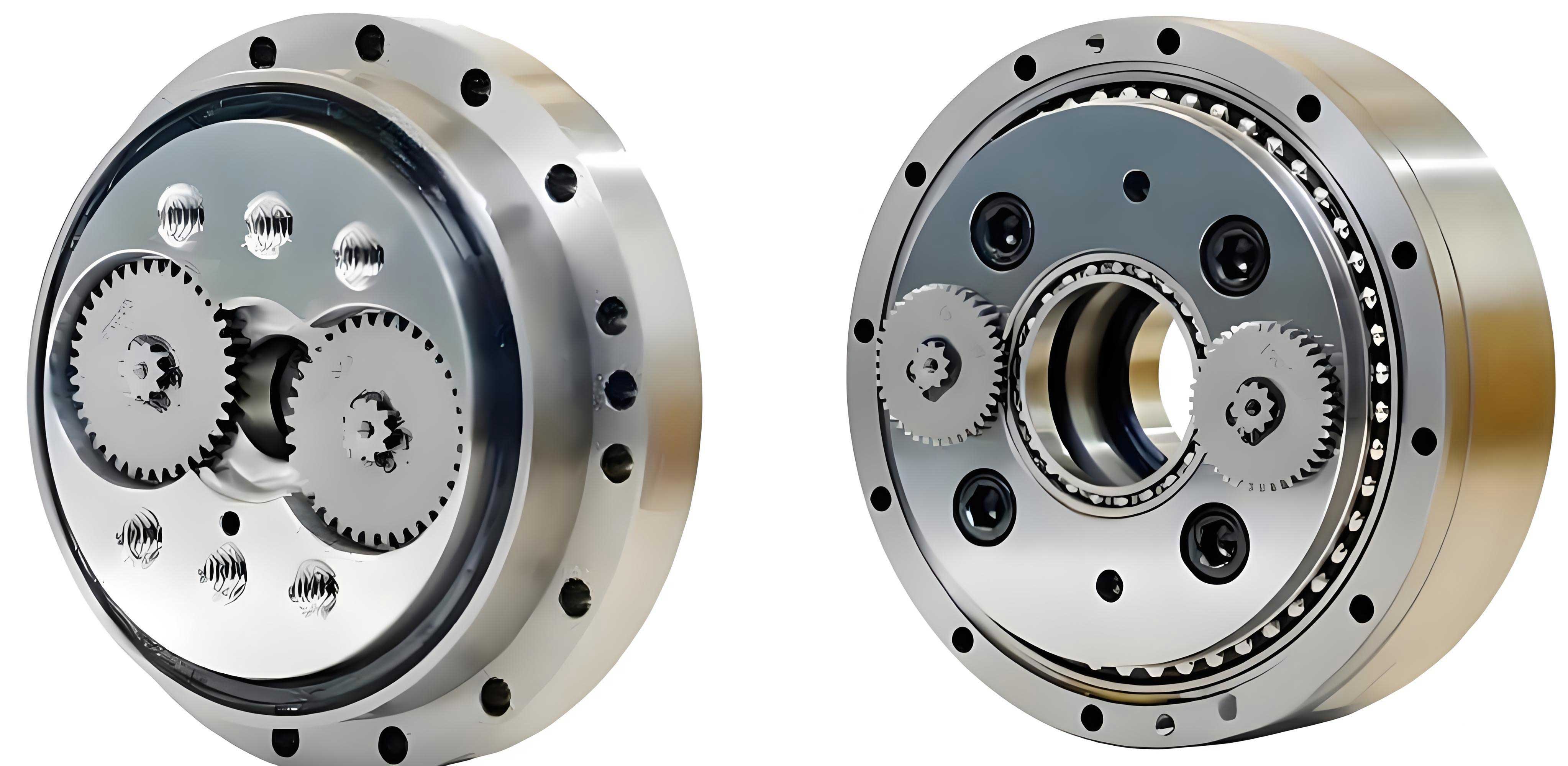
The reliability of industrial robots is fundamentally dependent on the health of their core components. Among these, the Rotary Vector (RV) reducer is a critical element, prized for its compact structure, large transmission ratio, and high precision. Ensuring its operational reliability is paramount for the safety and functionality of the entire robotic system. Consequently, effective condition monitoring and fault diagnosis for the RV reducer are of immense practical significance.
While data-driven artificial intelligence (AI) methods, such as convolutional neural networks (CNNs), have shown great promise in fault diagnosis, their practical deployment faces a significant hurdle: the scarcity of fault samples. In real-world engineering, RV reducers are typically maintained proactively, meaning genuine fault vibration data is extremely rare and difficult to obtain. This lack of labeled fault data severely limits the training and thus the diagnostic accuracy of AI models. To address this fundamental challenge of fault sample insufficiency, this work proposes a novel methodology: a dynamics model-driven intelligent fault diagnosis approach for the RV reducer. The core idea is to generate a comprehensive, high-fidelity fault sample library through numerical simulation of a high-precision dynamics model, which can then be used to train robust AI diagnostic models.
The proposed methodology follows a systematic, three-stage workflow. First, a high-fidelity translational-torsional coupled dynamic model of a healthy RV reducer is established. Second, mathematical models of specific gear faults are developed and integrated into the healthy dynamic model to simulate faulty conditions and generate vast amounts of synthetic vibration data. Finally, this synthetic fault sample library is used to train an AI classifier (e.g., a CNN), which is then validated using real-world experimental data from an RV reducer test rig to diagnose unknown faults.
1. Development of the RV Reducer Nonlinear Dynamic Model
1.1 Dynamic Modeling Assumptions and Coordinate Systems
The RV reducer is a two-stage precision speed reducer consisting of a first-stage planetary gear train (sun gear, planet gears) and a second-stage cycloid-pin mechanism (crank shafts, cycloid gears, pin wheel), with the output through a carrier. A 26-degree-of-freedom (DOF) lumped-parameter model is established, considering time-varying mesh stiffness, bearing support stiffness, and damping. The following assumptions are made:
- Identical components (planets, crank shafts, cycloid gears) have identical parameters and are evenly spaced.
- Gyroscopic effects are neglected.
- The input shaft speed is constant.
- Effects of gravity and friction are neglected.
To facilitate the formulation, three types of coordinate systems are defined: a fixed inertial frame \(OXY\), a central component frame that rotates with the carrier/output, and planet component frames that orbit the center.
1.2 Kinematic Acceleration Analysis
Since the equations of motion are formulated in rotating coordinate frames, the absolute acceleration of component mass centers must be properly expressed. For a central component (e.g., sun gear, carrier) with coordinates \((x_i, y_i)\) in its rotating frame rotating at \(\dot{\beta}\), the absolute acceleration components in the rotating frame are:
$$a_{ix} = \ddot{x}_i – 2\dot{\beta}\dot{y}_i – \dot{\beta}^2 x_i – \ddot{\beta} y_i$$
$$a_{iy} = \ddot{y}_i + 2\dot{\beta}\dot{x}_i – \dot{\beta}^2 y_i + \ddot{\beta} x_i$$
For a planet component (e.g., planet gear, crank shaft, cycloid gear) whose frame orbits at radius \(R\) with angular speed \(\dot{\beta}\), the absolute acceleration components are:
$$a_{jx} = \ddot{x}_j – 2\dot{\beta}\dot{y}_j – \dot{\beta}^2 x_j – \ddot{\beta} y_j – R\dot{\beta}^2$$
$$a_{jy} = \ddot{y}_j + 2\dot{\beta}\dot{x}_j – \dot{\beta}^2 y_j + \ddot{\beta} x_j – R\ddot{\beta}$$
1.3 Relative Displacements and Velocities at Mesh/Contact Points
The dynamic interactions are governed by the relative motions at gear meshes and bearing contacts. Key relative displacements (\(\delta\)) and their time derivatives (velocities, \(v\)) are formulated.
Sun-Planet Mesh: The relative displacement along the line of action is:
$$\delta_{si} = (x_s \cos\varphi_{si} + y_s \sin\varphi_{si} + r_s\theta_s) – (x_{pi} \cos\alpha_s – y_{pi} \sin\alpha_s + r_{pi}\theta_{pi})$$
where \(\varphi_{si} = \psi_i + \alpha_s\), \(\psi_i\) is the planet position angle, and \(\alpha_s\) is the pressure angle. A backlash function \(f(\delta_{si}, b)\) is applied to model gear clearance.
Crank Shaft-Cycloid Gear Bearing Contact: The relative displacements in the local x and y directions are:
$$\delta_{HiCjx} = x_{Hi} + e\theta_{Hi} \sin\psi_{Hi}^{Cj} – x_{Cj} \cos\psi_{Hi}^{Cj} – y_{Cj} \sin\psi_{Hi}^{Cj}$$
$$\delta_{HiCjy} = y_{Hi} – e\theta_{Hi} \cos\psi_{Hi}^{Cj} – x_{Cj} \sin\psi_{Hi}^{Cj} + y_{Cj} \cos\psi_{Hi}^{Cj} – r_H\theta_{Cj}$$
Crank Shaft-Carrier/Output Bearing Contact:
$$\delta_{iox} = x_{Hi} – x_o \cos\psi_{CHi} + y_o \sin\psi_{CHi}$$
$$\delta_{ioy} = y_{Hi} – x_o \sin\psi_{CHi} – y_o \cos\psi_{CHi} – r_H\theta_o$$
Cycloid Gear-Pin Wheel Mesh: The relative displacement along the cycloid-pin contact normal is a complex function involving the cycloid gear coordinates \((x_{Cj}, y_{Cj}, \theta_{Cj})\), the pin wheel coordinates, and the cycloid gear’s rotation relative to the pins.
$$\delta_{Cjr} = (x_{Cj}\sin\beta + y_{Cj}\cos\beta) – e\theta_{Cj}\sin(\beta – \theta_{Cj}) – (x_{or}\sin\beta + y_{or}\cos\beta) + r_c\theta_c\cos\beta$$
Pin Wheel-Housing Support: Assuming the housing is fixed, the relative displacement of the pin wheel is simply its translational coordinates.
1.4 Derivation of System Equations of Motion
The system’s kinetic energy \(T\), potential energy \(U\), and dissipation function \(D\) are constructed by summing contributions from all components and their interactions (gear meshes, bearing contacts). The generalized coordinates vector \(\mathbf{q}\) includes translational and rotational DOFs for the sun gear, planet gears, crank shafts, cycloid gears, carrier/output, and pin wheel. Applying the Lagrange equation:
$$\frac{d}{dt}\left(\frac{\partial T}{\partial \dot{q}_k}\right) – \frac{\partial T}{\partial q_k} + \frac{\partial U}{\partial q_k} + \frac{\partial D}{\partial \dot{q}_k} = F_k$$
yields the complete set of 26 second-order nonlinear differential equations of motion for the RV reducer system. \(F_k\) represents the generalized forces, primarily the input torque on the sun gear and the load torque on the carrier/output.
1.5 Model Updating for Fidelity
To ensure the simulated dynamics closely match real-world behavior, the initial model must be updated or tuned. The Pearson Correlation Coefficient (PCC) is used as a similarity metric between simulated and experimentally measured healthy state vibration signals. The model parameters (e.g., stiffness, damping) are iteratively adjusted until the PCC exceeds a predefined threshold (e.g., 0.7), ensuring a model of sufficient fidelity for reliable fault sample generation.
2. Modeling of Gear Faults via Time-Varying Mesh Stiffness (TVMS)
Gear faults are introduced into the dynamic model by modifying the TVMS, a primary internal excitation. The potential energy method is employed to calculate the mesh stiffness, considering Hertzian contact stiffness \(k_h\), bending stiffness \(k_b\), shear stiffness \(k_s\), and axial compressive stiffness \(k_a\). The total effective mesh stiffness for a sun-planet pair is:
$$\frac{1}{k_{sp}} = \frac{1}{k_{h}} + \frac{1}{k_{b1}} + \frac{1}{k_{b2}} + \frac{1}{k_{s1}} + \frac{1}{k_{s2}} + \frac{1}{k_{a1}} + \frac{1}{k_{a2}} + \frac{1}{k_{f1}} + \frac{1}{k_{f2}}$$
For double-tooth contact regions, the stiffnesses are summed in parallel.
2.1 TVMS for Healthy Gear
The stiffness is calculated by integrating along the tooth profile. The moments of area \(I_x\) and area \(A_x\) of the tooth section at a distance \(x\) from the base are key. The healthy TVMS exhibits characteristic fluctuations due to the changing number of tooth pairs in contact (varying between 1 and 2).
2.2 TVMS for Worn Gear
Non-uniform tooth wear, typically minimal at the pitch point, is modeled. The wear depth \(h_w(\alpha)\) at a pressure angle \(\alpha\) is calculated based on an Archard wear model. The worn tooth profile modifies the effective tooth thickness, altering the sectional area and moment of inertia used in the stiffness calculation:
$$A_x = (h_x – h_w \cos\alpha) L$$
$$I_x = \frac{1}{12} (h_x – h_w \cos\alpha)^3 L$$
This results in a reduction of TVMS, with the reduction magnitude dependent on the wear severity.
2.3 TVMS for Cracked Gear
A root crack is modeled as propagating linearly from the fillet. Four scenarios are considered based on crack length \(q_1\) (before crossing the centerline) and \(q_2\) (after crossing), and crack angle \(\nu\). The crack reduces the effective area and moment of inertia of the tooth root section. For example, in one scenario:
$$A_x = (h_a + h_x) L \quad \text{for} \quad x > d_a$$
$$I_x = \frac{1}{12} (h_a + h_x)^3 L \quad \text{for} \quad x > d_a$$
where \(h_a\) is the additional loss of tooth thickness due to the crack. The TVMS drops significantly, especially when the cracked section is under load.
2.4 TVMS for Broken Tooth
A broken tooth is modeled as a complete loss of load-carrying capacity. During the double-tooth contact period, if one tooth is broken, the total mesh stiffness equals that of the single healthy tooth pair. During the single-tooth contact period where the broken tooth is supposed to carry the load, the effective mesh stiffness becomes zero, representing a severe periodic impact excitation in the dynamic model.
3. Diagnosis Efficacy Analysis: From Simulation to Experiment
3.1 Generation of Simulated Fault Samples
Six health states are defined for the RV reducer: Healthy (T1), Broken Tooth (T2), Wear (T3), Crack (T4), combined Broken Tooth and Wear (T5), and combined Broken Tooth, Wear, and Crack (T6). The corresponding fault TVMS models are integrated into the updated dynamic model. The model is solved numerically to generate 60-second long vibration acceleration signals for each state at a sampling frequency of 48 kHz. To mimic real noisy environments, white Gaussian noise is added to the simulated signals. Each long signal is segmented into non-overlapping samples of 8000 data points.
| Fault Type | Label | Description |
|---|---|---|
| T1 | 1 | Healthy State |
| T2 | 2 | Broken Tooth |
| T3 | 3 | Gear Wear |
| T4 | 4 | Root Crack |
| T5 | 5 | Broken Tooth + Wear |
| T6 | 6 | Broken Tooth + Wear + Crack |
3.2 Fault Recognition using a Convolutional Neural Network (CNN)
A 1D CNN is chosen as the intelligent classifier. The architecture is designed to extract local temporal features from the vibration signals.
| Layer Type | Parameters |
|---|---|
| 1D Convolution | Kernel:5, Stride:2, Padding:2, Activation: ReLU |
| 1D Convolution | Kernel:3, Stride:1, Padding:1, Activation: ReLU |
| Max Pooling | Kernel:2 |
| 1D Convolution | Kernel:3, Stride:1, Padding:1, Activation: ReLU |
| Max Pooling | Kernel:2 |
| Flatten | – |
| Dropout | Rate: 0.9 |
| Fully Connected | Input:12800, Output:6400, Activation: ReLU |
| Dropout | Rate: 0.5 |
| Fully Connected | Input:6400, Output:320, Activation: ReLU |
| Output Layer | Input:320, Output:6, Activation: Softmax |
The model is trained exclusively on the 1560 simulated samples (260 per fault state). It is then tested on a hold-out set of 600 simulated samples (100 per state) to evaluate its performance on synthetic data.
3.3 Validation with Experimental Data
To validate the practical viability of the method, an RV reducer test rig is established. Vibration data is collected for four real fault conditions: wear, crack, broken tooth, and a compound fault. These real-world signals, completely unseen during the CNN’s training on simulated data, are segmented into 300 samples and used as a final validation set.
The CNN, trained purely on dynamics-model-generated data, achieves high classification accuracy on both the simulated test set and, crucially, on the experimental validation set. The results demonstrate that the fault features learned from the high-fidelity simulations are transferable to real vibration signals.
| Fault Type | Train Samples | Validation Samples | Best Accuracy (%) | Average Accuracy (%) |
|---|---|---|---|---|
| T1 (Healthy) | 260 | 50 | 100 | 99.2 |
| T2 (Broken Tooth) | 260 | 50 | 100 | 99.6 |
| T3 (Wear) | 260 | 50 | 100 | 98.8 |
| T4 (Crack) | 260 | 50 | 100 | 99.6 |
| T5 (Compound 1) | 260 | 50 | 100 | 100 |
| T6 (Compound 2) | 260 | 50 | 100 | 99.2 |
4. Conclusions
This work successfully proposes and validates a dynamics model-driven fault diagnosis methodology for the RV reducer, effectively addressing the critical issue of fault sample scarcity in AI-based diagnostics.
- High-Fidelity Modeling: A detailed 26-DOF nonlinear dynamic model of the RV reducer was developed and updated using correlation metrics to ensure its fidelity to real system dynamics.
- Fault Mechanism Integration: Mathematical models for key gear faults (wear, crack, breakage) were developed based on TVMS calculations and seamlessly integrated into the healthy dynamic model, enabling the simulation of realistic faulty vibration responses.
- Data Generation and AI Training: The fault-embedded dynamic model served as a high-precision simulator to generate a comprehensive library of labeled fault vibration data. This synthetic dataset was used to successfully train a CNN model.
- Practical Validation: The CNN, trained solely on simulation data, demonstrated high diagnostic accuracy when applied to real experimental data from an RV reducer test rig. This proves the transferability of knowledge from the simulation domain to the physical domain and validates the core premise of the methodology.
In summary, the dynamics model-driven approach provides a viable and powerful solution to overcome the data bottleneck in intelligent fault diagnosis for critical components like the RV reducer. It paves the way for the development of robust, data-efficient diagnostic systems where physical fault data is limited or unavailable.