
The RV reducer, an advanced transmission mechanism derived from traditional cycloidal-pinwheel planetary drives, has garnered significant attention globally. This is due to its superior characteristics which address the shortcomings of conventional designs. The RV reducer boasts a compact size, light weight, a wide range of transmission ratios, long service life, stable precision retention, high efficiency, and smooth operation. These advantages make it the preferred choice for high-precision robotics worldwide, alongside applications in machine tools, medical detection equipment, and satellite reception systems. The performance and reliability of an RV reducer are critically dependent on its key components, among which the angular contact ball bearings play a pivotal role. This article delves into the operational principles of the RV reducer, conducts a detailed theoretical load calculation for its main angular contact ball bearings, and validates these calculations through finite element simulation analysis.
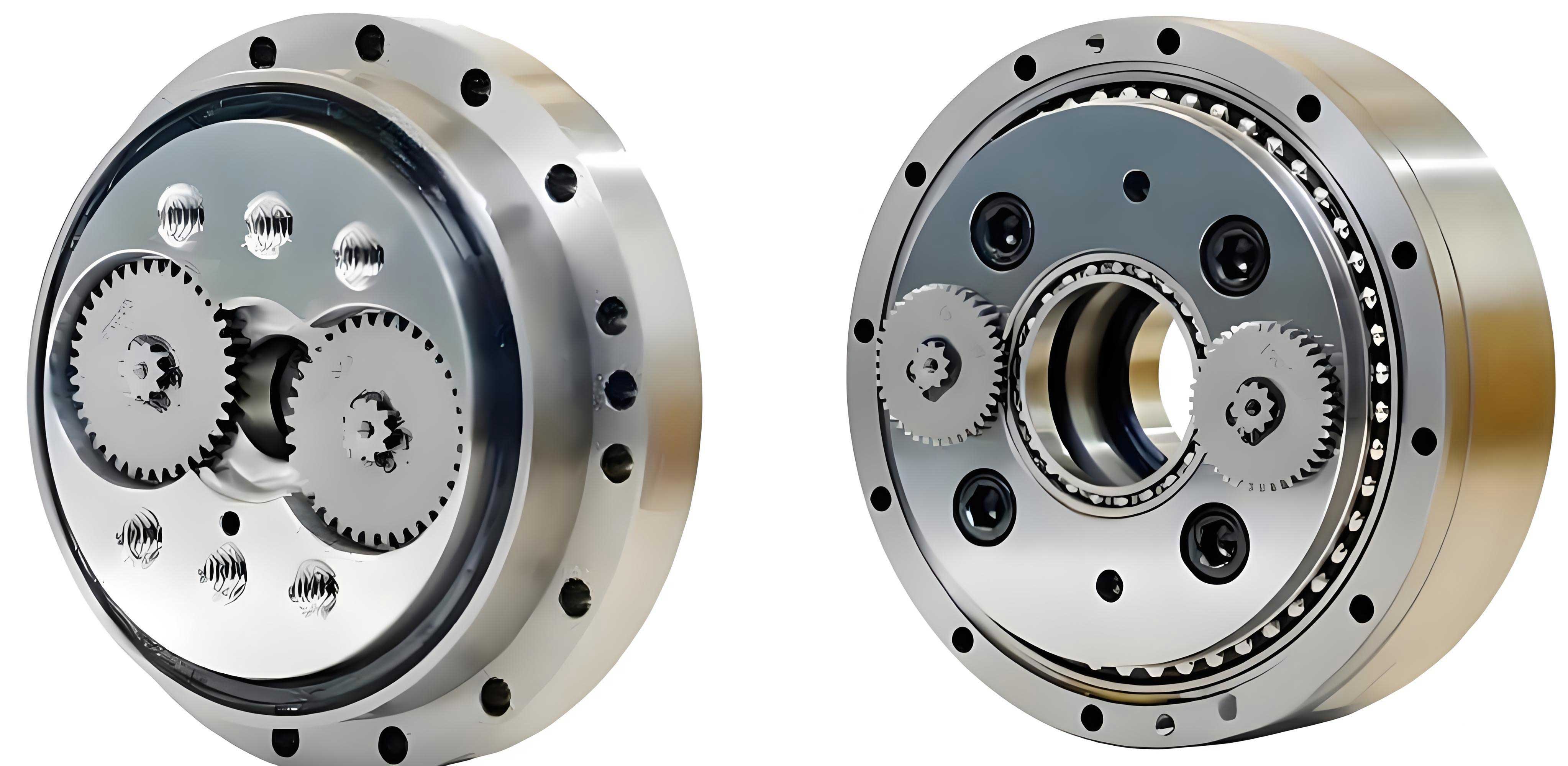
Introduction to the RV Reducer
Structural Composition
The C-series RV reducer is a two-stage, closed differential gear system. It uniquely combines a primary involute planetary gear stage with a secondary cycloidal-pinwheel stage in a series configuration, though their interaction is more complex than simple summation. The main structural components are:
- Gear Shaft (Input Shaft & Sun Gear): This integrated component serves as the power input, meshing with the planetary gears.
- Planetary Gears: Connected to the crankshafts via keys, these gears are uniformly distributed around the sun gear. Their primary functions are speed reduction and power splitting, transmitting the input power to two parallel cycloidal drives. Together with the gear shaft, they form the first reduction stage.
- Crankshafts: These are eccentrically mounted shafts. One end is keyed to a planetary gear, sharing its motion, while the other end is connected to the planet carrier via support bearings. The crankshaft’s rotation drives the cycloidal disks.
- Cycloidal Disks: Two identical cycloidal disks are mounted on the eccentric portions of the crankshafts via crossed roller bearings (often referred to as “tapered” or “turntable” bearings in this context). They mesh with the pinwheel. The two disks are installed 180 degrees out of phase to balance radial forces.
- Pinwheel (Needle Gear): Typically stationary, it consists of a pin housing (or ring) and multiple needle pins inserted into it. The pins engage with the teeth of the cycloidal disks.
- Planet Carrier (Output Flange): This is the output member of the RV reducer. It is driven by the crankshafts via support bearings and provides the final, low-speed, high-torque output.
- Angular Contact Ball Bearings (Main Bearings): These are typically thin-section bearings that support the entire rotating assembly of the RV reducer (planet carrier and attached components). They must withstand combined radial, axial, and moment loads, making their analysis crucial.
Working Principle
The power flow in an RV reducer is a two-stage process with a speed conversion mechanism. Assuming clockwise input rotation:
- First Stage (Involute Planetary): The motor drives the gear shaft (sun gear) clockwise. The planetary gears, meshing with the sun gear, rotate counterclockwise on their own axes while revolving clockwise around the sun gear. This planetary motion provides the first level of speed reduction. The crankshafts, rigidly connected to the planetary gears, inherit this compound motion.
- Second Stage (Cycloidal-Pinwheel): The eccentric motion of the crankshafts forces the two cycloidal disks to undergo an eccentric revolution. Due to the meshing constraint with the fixed pinwheel’s needle pins and the unique shape of the cycloidal tooth profile, this forced eccentric revolution causes the cycloidal disks to rotate slowly in the opposite direction (clockwise) about their own centers. This slow rotation is the self-rotation of the cycloidal disks.
- Output: The crankshafts, connected to the planet carrier via support bearings, transmit the self-rotation of the cycloidal disks to the planet carrier at a 1:1 ratio. Consequently, the planet carrier rotates clockwise at a greatly reduced speed, achieving the second and final stage of reduction. The total reduction ratio is the product of the first-stage planetary ratio and the high-ratio second-stage cycloidal drive.
The unique design of the RV reducer results in exceptional torque density, stiffness, and torsional backlash performance.
Theoretical Load Calculation for Angular Contact Ball Bearings
The angular contact ball bearings in an RV reducer are subjected to complex loading conditions stemming from the input torque, gear reaction forces, and external moments. A static load analysis under the condition of maximum instantaneous input torque is essential for evaluating bearing life and system rigidity.
Bearing Load Capacity Calculation
Consider a pair of angular contact ball bearings (e.g., model 76182B, contact angle $$ \alpha = 40^\circ $$, number of balls $$ Z = 51 $$) supporting the RV reducer’s output system. The load diagram is simplified as two bearings supporting a shaft subjected to radial gear forces, an input torque-induced tangential force, an external axial thrust, and an external bending moment at a specific point. The following parameters are known:
| Parameter | Symbol | Value |
|---|---|---|
| Distance from Bearing 1 to load point | a | 165.23 mm |
| Distance from Bearing 2 to load point | b | 40.83 mm |
| Input pinion radius | r₁ | 14.875 mm |
| Sun gear radius (for reaction calc) | r₂ | 98 mm |
| Max. instantaneous input torque | Timax | 20.24 Nm |
| Max. allowable external moment | Mc | 4900 Nm |
| Max. allowable external thrust | FA | 13.72 kN |
| Gear pressure angle | αg | 20° |
1. Calculate Forces from Input Torque:
Tangential force on input pinion:
$$ F_T = \frac{T_{i}^{max}}{r_1} = \frac{20.24}{0.014875} \approx 1360.54 \text{ N} $$
Radial component from gear meshing:
$$ F_R = F_T \cdot \tan(\alpha_g) = 1360.54 \cdot \tan(20^\circ) \approx 495.2 \text{ N} $$
2. Calculate Bearing Radial Reactions (Fr1, Fr2):
Using static equilibrium equations in two orthogonal planes (XOY and XOZ) considering the radial force F_R and the external moment M_c, we solve for the radial reaction components at each bearing. The system of equations derived from force and moment balance is:
For the plane containing F_R and M_c:
$$ \frac{F_{Rr1} + F_{Rr2}}{2} (a + b) + F_{Rr1} \cdot b = M_c + F_R \cdot r_2 $$
$$ F_{Rr1} + F_{Rr2} = F_R $$
For the plane containing F_T:
$$ \frac{F_{Tr1} + F_{Tr2}}{2} (a + b) = F_T \cdot b $$
$$ F_{Tr1} + F_{Tr2} = F_T $$
Solving these equations yields the component radial forces. The total radial load on each bearing is the vector sum:
$$ F_{r1} = \sqrt{F_{Rr1}^2 + F_{Tr1}^2} $$
$$ F_{r2} = \sqrt{F_{Rr2}^2 + F_{Tr2}^2} $$
The calculated results are:
$$ F_{r1} \approx 17.35 \text{ kN}, \quad F_{r2} \approx 17.88 \text{ kN} $$
3. Calculate Bearing Axial Loads (Fa1, Fa2):
For angular contact ball bearings, an applied radial load induces a derived axial force (Fd). For a 40° contact angle bearing, a common approximation is Fd ≈ 1.14 Fr.
$$ F_{d1} = 1.14 \times F_{r1} \approx 19.78 \text{ kN} $$
$$ F_{d2} = 1.14 \times F_{r2} \approx 20.38 \text{ kN} $$
The external axial load FA = 13.72 kN acts on the shaft. To determine the final axial load on each bearing, we analyze equilibrium:
$$ F_A + F_{d1} = 13.72 + 19.78 = 33.5 \text{ kN} > F_{d2} = 20.38 \text{ kN} $$
This indicates Bearing 2 is “tightened” and Bearing 1 is “relaxed.” Therefore:
$$ F_{a1} = F_{d1} = 19.78 \text{ kN} $$
$$ F_{a2} = F_A + F_{d1} = 33.5 \text{ kN} $$
Internal Load Distribution and Contact Stress Calculation
Using the calculated radial and axial loads, the internal load distribution among the rolling elements can be determined. The load distribution is governed by the relative magnitudes of axial and radial load, characterized by the parameter $$ e = \frac{F_a}{F_r} $$.
For Bearing 1:
$$ e_1 = \frac{F_{a1}}{F_{r1}} = \frac{19.78}{17.35} \approx 1.140 $$
For Bearing 2:
$$ e_2 = \frac{F_{a2}}{F_{r2}} = \frac{33.5}{17.88} \approx 1.873 $$
Given the contact angle α=40°, these values are used with standard load distribution integrals (Jr(ε), Ja(ε)) to find the load distribution factor ε and the maximum rolling element load Qmax.
$$ Q_{max} = \frac{F_r}{Z \cdot J_r(\varepsilon) \cos \alpha} $$
For the analyzed bearings, the results are:
$$ \varepsilon_1 \approx 0.7155, \quad Q_{1}^{max} \approx 1766.92 \text{ N} $$
$$ \varepsilon_2 \approx 1.2288, \quad Q_{2}^{max} \approx 1980.53 \text{ N} $$
The load on any other ball at angle φ from the position of maximum load is given by:
$$ Q(\phi) = Q_{max} \left[ 1 – \frac{1}{2\varepsilon}(1 – \cos \phi) \right]^{1.5} $$
The load distribution for each bearing is summarized in the table below. The load zone for Bearing 1 is limited (load angle ~115.5°), while for Bearing 2, all balls are under load due to the higher axial load ratio.
| φ (deg) | Q(φ) for Bearing 1 (N) | Q(φ) for Bearing 2 (N) |
|---|---|---|
| 0 | 1766.92 | 1980.53 |
| 7.06 | 1752.90 | 1971.37 |
| 14.12 | 1711.28 | 1944.13 |
| 21.18 | 1643.34 | 1899.46 |
| 28.24 | 1551.19 | 1838.45 |
| 35.29 | 1437.67 | 1762.55 |
| 42.35 | 1306.30 | 1673.57 |
| 49.41 | 1161.10 | 1573.58 |
| 56.47 | 1006.54 | 1464.87 |
| 63.53 | 847.35 | 1349.86 |
| 70.59 | 688.42 | 1231.06 |
| 77.65 | 534.61 | 1110.94 |
| 84.71 | 390.71 | 991.88 |
| 91.76 | 261.33 | 876.12 |
| 98.82 | 150.98 | 765.66 |
| 105.88 | 64.42 | 662.23 |
| 112.94 | 8.64 | 567.23 |
| 120.00 | 0.00 | 481.72 |
| 127.06 | 0.00 | 406.39 |
| 134.12 | 0.00 | 341.58 |
| 141.18 | 0.00 | 287.32 |
| 148.23 | 0.00 | 243.34 |
| 155.29 | 0.00 | 209.19 |
| 162.35 | 0.00 | 184.30 |
| 169.41 | 0.00 | 168.09 |
| 176.47 | 0.00 | 160.12 |
Hertzian Contact Stress and Deformation:
The contact between the ball and the outer raceway (typically the more critical contact) is analyzed using Hertzian theory. For the point of maximum load Qmax, the semi-major (a) and semi-minor (b) axes of the contact ellipse, the maximum contact stress (σmax), and the mutual approach (δ) are calculated. The general formulas involve the material properties (modulus of elasticity E, Poisson’s ratio ν), the principal curvatures of the contacting bodies (Σρ), and elliptic integrals. Simplified relations using coefficients a*, b*, δ* derived from the curvature difference are:
Contact ellipse semi-axes:
$$ a = a^* \left( \frac{Q}{\Sigma \rho} \right)^{1/3} $$
$$ b = b^* \left( \frac{Q}{\Sigma \rho} \right)^{1/3} $$
Maximum contact stress:
$$ \sigma_{max} = \frac{3Q}{2\pi a b} $$
Mutual approach (deformation):
$$ \delta = \delta^* \left( \frac{Q^2}{\Sigma \rho} \right)^{1/3} $$
For the subject bearings, the calculated results for the outer race contact are:
| Parameter | Bearing 1 | Bearing 2 |
|---|---|---|
| Semi-major axis, a (mm) | 1.5635 | 1.6241 |
| Semi-minor axis, b (mm) | 0.2233 | 0.2319 |
| Max. contact stress, σmax (MPa) | 2416.52 | 2510.22 |
| Contact deformation, δ (mm) | 0.0159 | 0.0171 |
The calculated contact stresses are well below the yield strength of bearing steel (typically > 4200 MPa). For rolling bearings, a contact stress below 1500-2000 MPa is often associated with very long, theoretically infinite fatigue life. Therefore, the initial geometric design of the bearings appears adequate for the load conditions within this RV reducer system.
Finite Element Simulation Analysis
To validate the theoretical calculations and gain further insight into the stress state, a Finite Element Analysis (FEA) was conducted. Given that the angular contact ball bearing in an RV reducer is a large, thin-walled component with many rolling elements, analyzing the entire assembly is computationally expensive. Since the most critical location is the contact under the maximum load, the FEA model was simplified to a single ball-in-raceway contact pair, representing the condition at the position of maximum load (φ = 0°).
Model Setup
A three-dimensional solid model of the bearing’s critical section (inner race segment, ball, and outer race segment) was created based on the geometry of bearing 76182B. The following steps were taken in the simulation pre-processor:
- Material Properties: Standard bearing steel (e.g., AISI 52100) properties were assigned: Young’s Modulus E = 210 GPa, Poisson’s ratio ν = 0.3.
- Constraints: The outer raceway was assigned a fixed constraint, simulating its housing fit. The inner raceway was constrained with a cylindrical support allowing only rotation about the bearing axis, simulating its connection to the rotating planet carrier of the RV reducer.
- Contact Definition: A surface-to-surface contact algorithm was established between the ball and both raceways. A “Penalty” formulation was used for both normal and tangential behavior. Appropriate normal and tangential penalty factors were selected to ensure convergence and reasonable contact stiffness.
- Loading: The calculated radial (Fr) and axial (Fa) loads for Bearing 1 and Bearing 2 were applied separately as pressure/force loads on the inner raceway in the appropriate directions, representing the loads transmitted from the RV reducer’s internal mechanism.
- Meshing: A refined, structured hex-dominant mesh was generated, with particularly high density in the anticipated contact regions to accurately capture stress gradients.
Simulation Results and Comparison
The nonlinear static structural analysis was solved. The primary outputs of interest were the contact force at the single ball-raceway interface and the resulting maximum contact stress.
For Bearing 1: The simulated contact force was 1757.82 N, and the maximum contact stress was 2362.89 MPa.
For Bearing 2: The simulated contact force was 1990.20 N, and the maximum contact stress was 2527.42 MPa.
The comparison between theoretical Hertzian calculations and FEA results is summarized below:
| Metric | Method | Bearing 1 | Bearing 2 |
|---|---|---|---|
| Contact Force (N) | Theory | 1766.92 | 1980.53 |
| FEA | 1757.82 | 1990.20 | |
| Max. Contact Stress (MPa) | Theory | 2416.52 | 2510.22 |
| FEA | 2362.89 | 2527.42 | |
| Error | Force | ~0.5% | ~0.5% |
| Stress | ~2.2% | ~0.7% |
The excellent agreement between the theoretical and simulation results validates the analytical load distribution model and the assumptions made in the FEA setup. The minor discrepancies can be attributed to simplifications in the analytical model (such as the approximation for derived axial force and the use of load distribution integrals) and the idealized conditions in the FEA (perfect geometry, simplified constraints, selected penalty factors). This correlation confirms that the proposed methods accurately reflect the operational state of the angular contact ball bearings within the RV reducer under the specified loading condition.
Discussion and Implications for RV Reducer Design
The successful analysis of the angular contact ball bearing loads has several important implications for the design and application of RV reducers.
1. Bearing Selection and Sizing: The process demonstrates a systematic approach to verifying that a selected bearing type and size (76182B) can withstand the combined loads generated by the RV reducer’s unique kinematics. The fact that the calculated contact stresses are significantly lower than the material’s yield strength and even below the threshold for very high-cycle fatigue indicates a conservative and reliable design margin. This is crucial for the long-term, maintenance-free operation expected in industrial robotics.
2. System Rigidity Consideration: The analysis assumes a rigid housing and support structure. In a real RV reducer, the high stiffness of the gearbox casing and precise mounting are essential to maintain this assumption. Any excessive system deflection would alter the load distribution on the bearings, potentially increasing the load on fewer rolling elements and raising local stresses. The preload applied during bearing installation in an RV reducer is a critical factor in establishing the initial stiffness and minimizing deflection under load.
3. Validation of Analytical Tools: The close match between classical Hertzian theory and modern FEA provides confidence in using both tools for rapid design iteration and detailed validation, respectively. The analytical method allows for quick load and life estimates during the initial design phase of the RV reducer. The FEA method, once calibrated as shown here, can be used to investigate more complex scenarios, such as the effect of housing deformations, thermal loads, or dynamic loading conditions specific to the robot’s duty cycle.
4. Focus on Maximum Loaded Element: The strategy of modeling only the most critically loaded ball-raceway contact pair for FEA proved effective. This significantly reduces computational time and complexity while still providing accurate stress data for the worst-case scenario. This approach is highly practical for engineering assessments of bearings in complex systems like the RV reducer.
Conclusion
This comprehensive analysis provides a detailed examination of the loading conditions within the critical angular contact ball bearings of an RV reducer. Beginning with an explanation of the RV reducer’s working principle and force transmission path, we derived the radial and axial loads acting on the main support bearings under a maximum instantaneous torque condition. Utilizing classical rolling bearing load distribution theory and Hertzian contact mechanics, we calculated the internal load distribution among the rolling elements and determined the maximum contact stress and deformation.
Subsequently, a finite element simulation of a simplified, single-ball contact model was performed. The remarkable agreement between the theoretical calculations and the FEA results—with errors in contact force and stress generally below 2.5%—strongly validates both the analytical model and the simulation parameters. This confirms that the bearing’s geometric design is suitable for the demanding application within the RV reducer, as the induced contact stresses are within safe limits for achieving long operational life.
This integrated approach, combining fundamental mechanical theory with advanced simulation, offers a robust framework for analyzing and verifying the performance of key components in precision transmission systems. For the RV reducer, understanding and validating the bearing loads is a cornerstone of ensuring the overall reliability, precision, and longevity that make it indispensable in advanced automation and robotics. The methodology established here can be directly applied to the analysis and selection of bearings for other high-performance RV reducer models and configurations.