
In the field of industrial robotics, the RV reducer stands as a critical component, directly influencing the precision and performance of robotic systems. One of its paramount performance metrics is the dynamic transmission accuracy, often quantified by the angular transmission error (ATE). This error is influenced by a multitude of factors, including the modification of the cycloidal gear profile, bearing clearances, and dimensional tolerances of components. In this study, we focus on investigating the significance of different bearing clearances on the ATE of an RV reducer. Utilizing a multi-body dynamics simulation model that incorporates nonlinear gear contact, cycloidal gear profile modification, and bearing clearances, we conduct a series of simulated orthogonal experiments. The aim is to discern the sensitivity and influence patterns of various bearing clearances on the ATE, thereby providing actionable insights for the design and manufacturing of RV reducers, particularly in optimizing bearing clearance through dimensional tolerance control.
The RV reducer, a type of precision cycloidal drive, is renowned for its high torque capacity, compact size, and high reduction ratio. Its dynamic performance, however, is susceptible to minute variations in assembly and component dimensions. The angular transmission error, defined as the difference between the theoretical and actual output rotation for a given input, is a key indicator of transmission precision. Factors such as gear tooth modifications, bearing internal clearances, and manufacturing errors collectively contribute to this error. Among these, bearing clearances—specifically those of the main bearing, the crankshaft support bearing, and the crankshaft swing-arm bearing—are known to have a substantial impact. However, the interactive effects and relative significance of these clearances under specific cycloidal gear modification conditions are not fully elucidated. This research addresses this gap by integrating virtual prototyping with statistical experimental design.
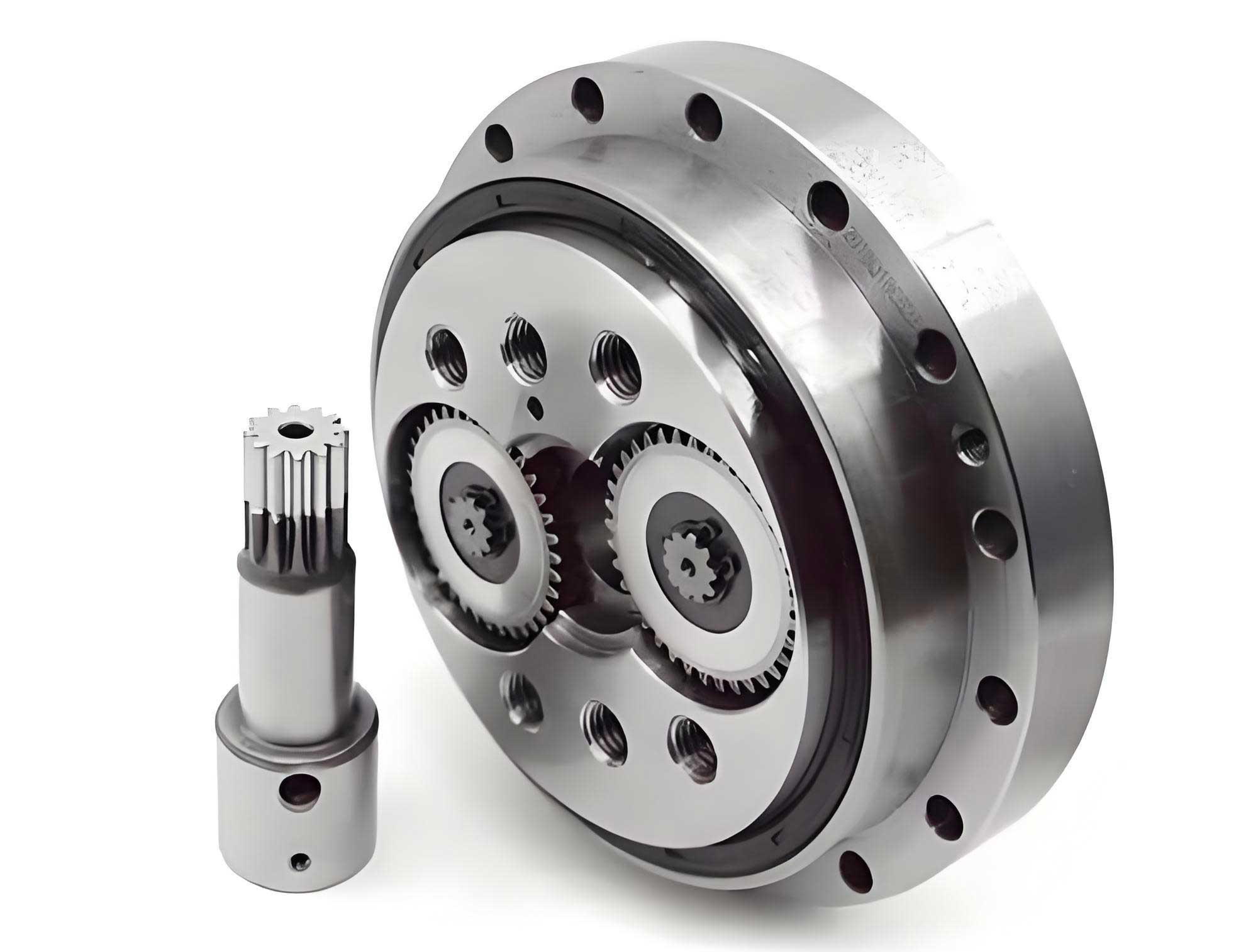
The internal structure of an RV reducer, such as the RV80E model studied here, features unique bearing arrangements. The main bearing is typically an angular contact ball bearing, where radial clearance arises from the dimensional tolerances of the planetary carrier, inner ring, balls, and the assembly preload. The crankshaft swing-arm bearing is often a needle roller bearing without inner and outer rings; its radial clearance is determined by the bore diameter of the cycloidal gear’s bearing hole, the journal diameter of the crankshaft, and the size tolerance of the needles. The crankshaft support bearing is a tapered roller bearing, where axial clearance adjustment via selective snap rings indirectly controls the radial clearance. These clearances are inherently tied to part tolerances and assembly precision. Indiscriminately tightening tolerances to minimize clearances for improved ATE is economically impractical. Therefore, understanding the sensitivity of ATE to each clearance type is crucial for establishing cost-effective tolerance specifications.
To systematically analyze the influence of bearing clearances, we employ an orthogonal experimental design coupled with multi-body dynamics simulation. Orthogonal design is a highly efficient method for multifactor experimentation, allowing the exploration of factor effects with a minimal number of trials while maintaining balanced and comparable data. For this study, the factors are the radial clearances of three bearings: the main bearing (Factor A), the crankshaft support bearing (Factor B), and the crankshaft swing-arm bearing (Factor C). Each factor is set at four levels, reflecting feasible ranges derived from high-precision bearing standards (e.g., NSK recommendations) and practical manufacturing capabilities for the RV reducer. The specific levels are detailed in Table 1.
| Level | Factor A: Main Bearing Clearance (µm) | Factor B: Crankshaft Support Bearing Clearance (µm) | Factor C: Crankshaft Swing-arm Bearing Clearance (µm) |
|---|---|---|---|
| 1 | 0 | 0 | 0 |
| 2 | 3 | 10 | 5 |
| 3 | 6 | 20 | 10 |
| 4 | 10 | 30 | 15 |
The response variable is the simulated angular transmission error of the RV reducer, measured in arc-minutes (‘). A smaller ATE indicates higher transmission precision. The orthogonal array L16(4^5) is selected, which accommodates up to five factors at four levels. Since we have three factors, the remaining columns are treated as error terms. The experimental layout and the corresponding simulation results are presented in Table 2. Each simulation run involves configuring the virtual RV reducer model with the specified clearance combination, applying a constant input speed, and measuring the output angle deviation over several cycles to compute the peak-to-peak ATE.
| Experiment No. | A: Main Bearing Clearance (µm) | B: Crankshaft Support Bearing Clearance (µm) | C: Crankshaft Swing-arm Bearing Clearance (µm) | Angular Transmission Error, x_i (‘) |
|---|---|---|---|---|
| 1 | 0 | 0 | 0 | 0.196 |
| 2 | 0 | 10 | 5 | 0.301 |
| 3 | 0 | 20 | 10 | 0.598 |
| 4 | 0 | 30 | 15 | 0.693 |
| 5 | 3 | 0 | 5 | 0.213 |
| 6 | 3 | 10 | 0 | 0.831 |
| 7 | 3 | 20 | 15 | 1.396 |
| 8 | 3 | 30 | 10 | 2.092 |
| 9 | 6 | 0 | 10 | 0.235 |
| 10 | 6 | 10 | 15 | 1.001 |
| 11 | 6 | 20 | 0 | 1.701 |
| 12 | 6 | 30 | 5 | 2.633 |
| 13 | 10 | 0 | 15 | 0.302 |
| 14 | 10 | 10 | 10 | 0.760 |
| 15 | 10 | 20 | 5 | 1.194 |
| 16 | 10 | 30 | 0 | 2.584 |
The foundation of our analysis is a high-fidelity multi-body dynamics model of the RV80E reducer. This virtual prototype incorporates several critical aspects: a precise cycloidal gear profile with combined modification (positive equidistance and negative offset), nonlinear contact forces between gear teeth (cycloidal gear and pin gear), and detailed bearing models with adjustable radial clearances. The equations of motion for the system are derived using Lagrange’s equations, accounting for the time-varying meshing stiffness and clearance-induced nonlinearities. The general form for a multi-body system can be expressed as:
$$ \mathbf{M}(\mathbf{q})\ddot{\mathbf{q}} + \mathbf{C}(\mathbf{q}, \dot{\mathbf{q}})\dot{\mathbf{q}} + \mathbf{K}(\mathbf{q})\mathbf{q} + \mathbf{F}_{nl}(\mathbf{q}, \dot{\mathbf{q}}) = \mathbf{Q}(t) $$
where \(\mathbf{M}\) is the mass matrix, \(\mathbf{C}\) is the damping matrix, \(\mathbf{K}\) is the stiffness matrix, \(\mathbf{F}_{nl}\) represents nonlinear forces from contacts and clearances, \(\mathbf{q}\) is the vector of generalized coordinates, and \(\mathbf{Q}\) is the vector of applied forces/torques. For the RV reducer, the angular transmission error \(\Delta\theta\) is computed as:
$$ \Delta\theta = \theta_{out} – \frac{\theta_{in}}{N} $$
where \(\theta_{out}\) is the actual output angle, \(\theta_{in}\) is the input angle, and \(N\) is the theoretical reduction ratio. The simulation model solves these equations numerically to obtain the dynamic response under steady-state operating conditions.
Following the simulation, we perform a comprehensive statistical analysis on the ATE data. The first step is range analysis (or extreme difference analysis), which provides an initial ranking of factor significance. For each factor \(i\), the range \(R_i\) is calculated as:
$$ R_i = \max(k_{i1}, k_{i2}, k_{i3}, k_{i4}) – \min(k_{i1}, k_{i2}, k_{i3}, k_{i4}) $$
where \(k_{ij}\) is the mean ATE for factor \(i\) at level \(j\). The values of \(k_{ij}\) are computed from Table 2 and summarized in Table 3. The range indicates the fluctuation amplitude of the indicator when the factor level changes; a larger range implies greater influence.
| Factor / Level | Level 1 | Level 2 | Level 3 | Level 4 | Range \(R_i\) |
|---|---|---|---|---|---|
| A: Main Bearing Clearance | 0.447 | 1.134 | 1.393 | 1.210 | 0.946 |
| B: Crankshaft Support Bearing Clearance | 0.237 | 0.723 | 1.222 | 2.001 | 1.764 |
| C: Crankshaft Swing-arm Bearing Clearance | 1.328 | 1.085 | 0.921 | 0.848 | 0.480 |
Based on the ranges, the order of factor significance is: B (crankshaft support bearing clearance) > A (main bearing clearance) > C (crankshaft swing-arm bearing clearance). This suggests that the support bearing clearance has the most pronounced effect on the ATE of the RV reducer, while the swing-arm bearing clearance has the least. However, range analysis is preliminary; a more rigorous method is analysis of variance (ANOVA).
ANOVA decomposes the total variation in the data into components attributable to each factor and experimental error. This allows for testing the statistical significance of each factor. The total sum of squares \(S_T\), factor sum of squares \(S_i\), and error sum of squares \(S_e\) are calculated as follows:
$$ S_T = \sum_{i=1}^{n} x_i^2 – \frac{(\sum_{i=1}^{n} x_i)^2}{n} $$
where \(n=16\) is the number of experiments. For each factor with \(t=4\) levels, the sum of squares is:
$$ S_i = \frac{1}{t} \sum_{j=1}^{t} K_{ij}^2 – \frac{(\sum_{i=1}^{n} x_i)^2}{n} $$
where \(K_{ij}\) is the sum of ATE values for factor \(i\) at level \(j\). The error sum of squares is \(S_e = S_T – S_A – S_B – S_C\). The degrees of freedom for the total is \(f_T = n-1 = 15\), for each factor \(f_i = \text{number of levels} – 1 = 3\), and for error \(f_e = f_T – \sum f_i = 6\). The mean square (variance estimate) for each source is \(MS_i = S_i / f_i\) and \(MS_e = S_e / f_e\). The F-statistic for each factor is \(F_i = MS_i / MS_e\), which is compared to critical F-values from statistical tables to determine significance. The detailed ANOVA table is presented in Table 4.
| Source of Variation | Sum of Squares (S) | Degrees of Freedom (f) | Mean Square (MS) | F-value | Significance |
|---|---|---|---|---|---|
| A: Main Bearing Clearance | 2.055 | 3 | 0.685 | 5.244 | Significant (*) |
| B: Crankshaft Support Bearing Clearance | 6.807 | 3 | 2.269 | 17.369 | Highly Significant (**) |
| C: Crankshaft Swing-arm Bearing Clearance | 0.543 | 3 | 0.181 | 1.387 | Not Significant |
| Error | 0.785 | 6 | 0.131 | ||
| Total | 10.190 | 15 |
Using significance levels α=0.05 and α=0.01, with critical values \(F_{0.05}(3,6)=4.53\) and \(F_{0.01}(3,6)=9.78\), we find that factor B is highly significant (F > 9.78), factor A is significant (4.53 < F < 9.78), and factor C is not significant (F < 4.53). This confirms the initial range analysis and provides statistical rigor. Furthermore, we compute the contribution rate \(\rho_i\) of each factor to the total variation:
$$ \rho_i = \frac{S_i}{S_T} \times 100\% $$
The contribution rates are: \(\rho_A = 20.17\%\), \(\rho_B = 66.80\%\), \(\rho_C = 5.33\%\), and \(\rho_{error} = 7.70\%\). This quantifies the dominance of the crankshaft support bearing clearance, accounting for over two-thirds of the observed variation in ATE for this RV reducer under the tested conditions.
To visualize the influence patterns, we plot the mean ATE against each factor level, as shown in Figure 1 (described narratively here since actual image insertion is limited to the provided link). For factor A (main bearing clearance), the ATE initially increases from 0.447′ at 0 µm to 1.393′ at 6 µm, then slightly decreases to 1.210′ at 10 µm. This non-monotonic behavior suggests a potential optimal range; excessive clearance might allow recentering that marginally reduces error. For factor B (crankshaft support bearing clearance), the ATE exhibits a strong, nearly linear increase from 0.237′ at 0 µm to 2.001′ at 30 µm. This clear trend underscores its critical impact; any increase in this clearance directly degrades the RV reducer’s transmission accuracy. For factor C (crankshaft swing-arm bearing clearance), the ATE surprisingly decreases from 1.328′ at 0 µm to 0.848′ at 15 µm. This inverse relationship implies that a modest increase in this clearance might slightly improve ATE, possibly by altering load distribution among the cycloidal gear teeth or mitigating binding effects. However, given its low significance, this effect is secondary.
The physical interpretation of these results lies in the load path and kinematic chain within the RV reducer. The crankshaft support bearing is crucial for maintaining the alignment and positional accuracy of the crankshaft, which directly affects the phase relationship between the cycloidal gears and the pin gear. Increased clearance here introduces larger radial play, amplifying kinematic errors that propagate to the output. The main bearing supports the planetary frame and carries significant loads; its clearance affects the system’s overall rigidity. The non-linear response may be due to a complex interplay between bearing deflection and gear mesh alignment. The swing-arm bearing, while important for cycloidal gear motion, operates under different constraints, and its clearance might have a compensatory effect on the meshing condition.
Based on these findings, we propose targeted design guidelines for bearing clearances in the RV reducer. First, the crankshaft support bearing clearance should be stringently controlled. In manufacturing, this translates to tight tolerances on the housing bore, bearing outer ring, and selective assembly of snap rings to minimize radial play. A design goal should be to keep this clearance as close to zero as practically feasible. Second, the main bearing clearance requires careful management. It should be controlled within a moderate range—perhaps between 3 µm and 6 µm for this specific RV reducer size—to avoid the region of peak ATE. Third, the crankshaft swing-arm bearing clearance can be relatively relaxed. This allows for wider manufacturing tolerances on the cycloidal gear bores and crankshaft journals, reducing production cost without compromising ATE performance. These recommendations must be balanced with other considerations like bearing life, thermal expansion, and lubrication.
In conclusion, this study demonstrates the efficacy of combining multi-body dynamics simulation with orthogonal experimental design to analyze the angular transmission error in an RV reducer. The virtual prototype, incorporating key nonlinearities, serves as a powerful tool for sensitivity analysis. The statistical results unequivocally identify the crankshaft support bearing clearance as the most significant factor affecting ATE, followed by the main bearing clearance, while the swing-arm bearing clearance has minimal impact under the given cycloidal gear modification. The derived influence patterns provide a scientific basis for designing dimensional tolerances for bearings in the RV reducer. By focusing control efforts on the most sensitive parameters, manufacturers can achieve the desired dynamic transmission accuracy in a cost-effective manner, enhancing the performance and competitiveness of industrial robots relying on these precision reducers. Future work could expand this approach to include interactions between factors, different load conditions, and the effects of thermal deformation on bearing clearances in the RV reducer.
The mathematical underpinnings of the orthogonal analysis can be further elaborated. The calculation of the factor sum of squares, for instance, for factor A involves the sums \(K_{A1}, K_{A2}, K_{A3}, K_{A4}\) which are the totals of ATE for experiments where factor A is at levels 1, 2, 3, and 4 respectively. From Table 2:
$$ K_{A1} = 0.196+0.301+0.598+0.693 = 1.788 $$
$$ K_{A2} = 0.213+0.831+1.396+2.092 = 4.532 $$
$$ K_{A3} = 0.235+1.001+1.701+2.633 = 5.570 $$
$$ K_{A4} = 0.302+0.760+1.194+2.584 = 4.840 $$
Then,
$$ S_A = \frac{1}{4}(1.788^2 + 4.532^2 + 5.570^2 + 4.840^2) – \frac{(16 \times \bar{x})^2}{16} $$
where \(\bar{x}\) is the overall mean ATE, calculated as \(\bar{x} = \frac{1}{16}\sum x_i = 1.046’\). This yields \(S_A = 2.055\), as shown. Similar calculations apply for other factors. The error mean square \(MS_e\) provides an estimate of the experimental variance, which is essential for F-tests. The non-significance of factor C suggests that its effect is within the noise level of the simulation and experimental error.
Moreover, the dynamics of the RV reducer can be modeled more deeply. The time-varying meshing stiffness \(k_m(t)\) between the cycloidal gear and the pin gear is a periodic function that depends on the number of teeth in contact. A simplified expression might be:
$$ k_m(t) = k_0 + \sum_{n=1}^{\infty} a_n \cos(n\omega_m t + \phi_n) $$
where \(k_0\) is the average stiffness, \(\omega_m\) is the meshing frequency, and \(a_n\) are Fourier coefficients. The bearing clearance introduces a piecewise-linear force-displacement relationship. For a radial clearance \(c_r\), the restoring force \(F_b\) in a bearing can be modeled as:
$$
F_b(\delta) =
\begin{cases}
0, & |\delta| \leq c_r/2 \\
k_b (\delta – c_r/2), & \delta > c_r/2 \\
k_b (\delta + c_r/2), & \delta < -c_r/2
\end{cases}
$$
where \(\delta\) is the radial displacement and \(k_b\) is the bearing stiffness. These nonlinearities are integrated into the multi-body model, making the simulation computationally intensive but accurate. The orthogonal design efficiently samples the clearance parameter space.
Finally, the implications for the design process of the RV reducer are substantial. By quantifying the sensitivity, engineers can perform tolerance allocation using methods like the Taguchi loss function or Monte Carlo simulation. The goal is to minimize the total cost of quality, which includes manufacturing cost (inversely related to tolerance tightness) and performance loss due to ATE. A composite objective function could be formulated:
$$ \min_{T_A, T_B, T_C} \left[ C_m(T_A, T_B, T_C) + \lambda \cdot L(\sigma_{ATE}) \right] $$
where \(T_i\) are tolerance bands for the clearances, \(C_m\) is manufacturing cost, \(\lambda\) is a weighting factor, \(L\) is the loss function (e.g., quadratic loss) depending on the standard deviation of ATE \(\sigma_{ATE}\), which can be estimated from the regression model derived from the orthogonal experiment. This systematic approach elevates the design of the RV reducer from empirical to analytical, ensuring robust performance in demanding robotic applications.