
The dynamic behavior of gear transmission systems is profoundly influenced by the periodic variation of gear mesh stiffness. During the meshing cycle of spur gears, the number of tooth pairs in simultaneous contact fluctuates, and the elastic teeth can be modeled as time-varying springs aligned with the line of action. This periodic elastic deformation is a primary excitation source for gear vibration and noise. Consequently, accurately calculating the time-varying meshing stiffness (TVMS) is of paramount importance for dynamic analysis, noise prediction, and durability assessment of gear drives. This work presents a detailed methodology for computing the TVMS of profile-shifted involute spur gears based on the Weber energy method, implemented through a parametric MATLAB program.
Traditional analytical methods for stiffness calculation, such as the Ishikawa formula, often simplify the tooth profile to a combination of rectangles and trapezoids. While the Weber method typically employs an accurate involute curve, the fillet or transition curve is frequently approximated. These simplifications can introduce non-negligible errors in the stiffness results. To enhance accuracy, this analysis utilizes precise mathematical models for both the involute profile and the trochoidal (or rounded) transition curve generated by the gear cutting process. The deformation under load is calculated using the Weber-Banaschek energy method, also referred to as the cantilever beam method in material mechanics. This method decomposes the total tooth deflection into three primary components: bending, shear, and axial compression of the tooth profile (including involute and transition curve); deflection of the gear body (or foundation); and local contact deformation at the meshing point.
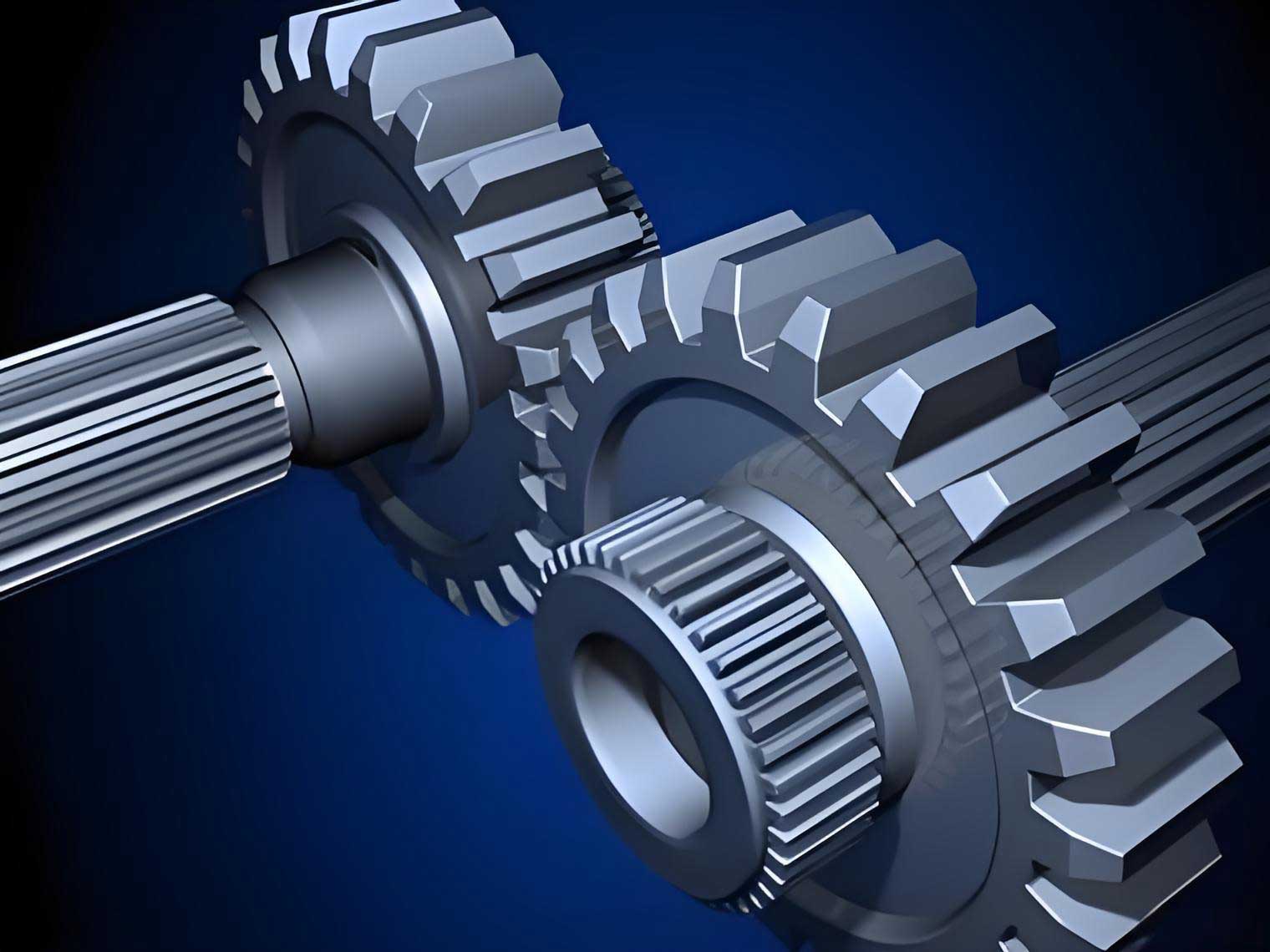
Precise Geometric Modeling of Spur Gears
Accurate geometric representation is the foundation for reliable stiffness calculation. For an involute spur gear, the profile from the start of active profile (SAP) to the tip circle is defined by the standard involute equations. Considering a point on the generating line, the parametric equations in a coordinate system with its origin at the gear center are:
$$
\begin{align}
x_{inv} &= r_b [\sin(\gamma – \delta) – \gamma \cos(\gamma – \delta)] \\
y_{inv} &= r_b [\cos(\gamma – \delta) + \gamma \sin(\gamma – \delta)]
\end{align}
$$
where $r_b$ is the base circle radius, and $\gamma$ and $\delta$ are intermediate parameters related to the involute development angle and the initial angle, respectively.
The transition curve between the involute profile and the root circle is modeled as the equidistant curve of the trochoid generated by the tip of the cutting tool (e.g., a rack cutter or hob). Its equations can be derived from the gear generation process. For a rack cutter with tip radius $\rho_a$, the transition curve coordinates $(x_{tr}, y_{tr})$ are given by:
$$
\begin{align}
x_{tr} &= (x_k + r_2 \varphi_2) \cos \varphi_2 – (y_k + r_2) \sin \varphi_2 \\
y_{tr} &= (x_k + r_2 \varphi_2) \sin \varphi_2 + (y_k + r_2) \cos \varphi_2
\end{align}
$$
where $r_2$ is the pitch radius of the gear being generated, $\varphi_2$ is the roll angle during generation, and $(x_k, y_k)$ are coordinates related to the cutter profile. This precise modeling of the entire active tooth flank allows for an accurate determination of the tooth’s cross-sectional properties as a function of height, which is critical for the subsequent deformation calculation.
Tooth Deformation Calculation via the Weber Energy Method
The tooth is modeled as a non-uniform cantilever beam fixed at the gear body. The beam is discretized into a series of small slices along its height. The total deformation $q_{12j}$ at a meshing point $j$ under a normal load $W_j$ is the sum of three parts: $q_{bj}$ (tooth bending, shear, axial compression), $q_{fej}$ (foundation deflection), and $q_{cj}$ (Hertzian contact deformation). The effective stiffness $K_j$ at point $j$ is then $K_j = W_j / q_{12j}$.
1. Tooth Profile Deformation ($q_{bj}$)
The tooth profile from the meshing point $j$ down to the base point $N$ (located on the root circle) is divided into $n$ micro-slices. For each slice $i$ with thickness $\delta_i$, average cross-sectional area $\bar{A}_i$, and average area moment of inertia $\bar{I}_i$ about the neutral axis, the contribution to deformation in the direction of $W_j$ is calculated. The load $W_j$ applied at an angle $\beta_j$ relative to the tooth centerline is resolved into components and a moment acting on each slice. The deformation $q_{bij}$ of slice $i$ due to the load at point $j$ is derived from beam theory:
$$
\begin{aligned}
q_{bij} &= \frac{W_j}{E_e \bar{A}_i} \delta_i \sin^2 \beta_j + \frac{12 W_j (1+\nu)}{5 E_e \bar{A}_i} \delta_i \cos^2 \beta_j \\
&+ \frac{W_j \cos^2 \beta_j}{E_e} \left( \frac{\delta_i^3 + 3\delta_i^2 L_{ij} + 3\delta_i L_{ij}^2}{3\bar{I}_i} \right) \\
&- \frac{W_j \sin \beta_j \cos \beta_j}{E_e} \left( \frac{\delta_i^2 Y_j + 2\delta_i Y_j L_{ij}}{2\bar{I}_i} \right)
\end{aligned}
$$
where $E_e$ is the effective Young’s modulus, $\nu$ is Poisson’s ratio, $L_{ij}$ is the distance from slice $i$ to the load point $j$ along the tooth axis, and $Y_j$ is the $y$-coordinate of point $j$. The total profile deformation is $q_{bj} = \sum_{i=1}^{n} q_{bij}$. The effective modulus $E_e$ depends on the tooth aspect ratio: $E_e = E/(1-\nu^2)$ for wide teeth ($b/s_p > 5$), and $E_e = E$ for narrow teeth, where $b$ is face width and $s_p$ is the tooth thickness at the pitch point.
2. Foundation Deformation ($q_{fej}$)
The deflection of the gear body supporting the tooth is calculated using formulas derived from elasticity theory, often incorporating factors proposed by O’Donnell. The expressions differ for wide and narrow teeth. For wide teeth:
$$
q_{fej} = \frac{W_j \cos^2 \beta_j}{E b (1-\nu^2)} \left[ \frac{16.67}{\pi} \left( \frac{L_f}{H_f} \right)^2 + \frac{2(1-\nu)-2\nu^2}{1-\nu^2} \frac{L_f}{H_f} + 1.534 \left( 1 + \frac{\tan^2 \beta_j}{2.4(1+\nu)} \right) \right]
$$
For narrow teeth:
$$
q_{fej} = \frac{W_j \cos^2 \beta_j}{E b} \left[ \frac{16.67}{\pi} \left( \frac{L_f}{H_f} \right)^2 + 2(1-\nu) \frac{L_f}{H_f} + 1.534 \left( 1 + \frac{\tan^2 \beta_j}{2.4(1+\nu)} \right) \right]
$$
Here, $H_f = 2 Y_N$ is the chordal thickness at the base point $N$ with coordinates $(X_N, Y_N)$, and $L_f = X_j – X_N – Y_j \tan \beta_j$ is the effective load arm for foundation deflection.
3. Contact Deformation ($q_{cj}$)
The local deformation due to Hertzian contact between two tooth surfaces is given by a semi-empirical formula based on Lundberg’s work:
$$
q_{cj} = \frac{1.275 W_j^{0.9}}{E_{12e}^{0.9} l^{0.8}}
$$
where $l$ is the length of contact (face width $b$ for perfect contact), and $E_{12e}$ is the combined effective modulus:
$$\frac{1}{E_{12e}} = \frac{1}{2}\left( \frac{1}{E_{1e}} + \frac{1}{E_{2e}} \right)$$
For a constant load $W_j$, this component is constant throughout the mesh cycle.
The total deformation at point $j$ is thus:
$$ q_{12j} = q_{bj} + q_{fej} + q_{cj} $$
| Deformation Component | Symbol | Governing Factors | Dependency on Load Point |
|---|---|---|---|
| Tooth Profile (Bending, Shear, Axial) | $q_{bj}$ | Tooth geometry, material ($E, \nu$), load angle $\beta_j$ | Strong function of position (via $\beta_j$, $L_{ij}$, $Y_j$) |
| Foundation Deflection | $q_{fej}$ | Gear body geometry, material, load arm $L_f$ | Function of position (via $\beta_j$, $L_f$) |
| Hertzian Contact | $q_{cj}$ | Material properties, face width, load magnitude | Constant for constant $W_j$ |
Mapping Relations and Stiffness Formulation for Spur Gears
The load angle $\beta_j$ is a crucial parameter. It is related to the pressure angle $\alpha_j$ at the contact point and the coordinates $(X_{Mj}, Y_{Mj})$ of point $j$ on the tooth profile. From geometric analysis:
$$ \beta_j = \alpha_j – \theta’ $$
where $\theta’ = \arctan(Y_{Mj}/X_{Mj})$, and $\alpha_j = \arccos(r_b / \overline{OM}_j)$ with $\overline{OM}_j = \sqrt{X_{Mj}^2 + Y_{Mj}^2}$.
Furthermore, the roll angle on the base circle corresponding to point $j$ is given by the involute function:
$$ \text{Roll Angle} = \operatorname{inv}(\alpha_j) + \alpha_j = \tan \alpha_j $$
This establishes a direct mapping between the contact point position $X_{Mj}$, the pressure angle $\alpha_j$, and the roll angle $\tan \alpha_j$. Therefore, the single-tooth stiffness $K_j$ can be expressed as a function of $\alpha_j$ or $\tan \alpha_j$, which is more convenient for analyzing stiffness variation over the meshing cycle of spur gears.
Determination of Single and Double Tooth Contact Regions
For spur gears with a transverse contact ratio $\varepsilon_{\alpha} > 1$, the meshing cycle alternates between double tooth pair contact (DTPC) and single tooth pair contact (STPC) regions. Identifying the boundaries of these regions is essential for calculating the mesh stiffness of the gear pair. The key points along the line of action are: the start of active profile (A), the start of the STPC region (B), the end of the STPC region (D), and the end of contact (E). Point C is the pitch point.
The radial distances from the gear centers to these boundary points are calculated using the law of cosines, based on the geometry of engagement. For example, for the driving gear at point B:
$$ r_{B1} = \sqrt{ \overline{CB}^2 + {r’_1}^2 – 2 \overline{CB} r’_1 \cos(\angle O_1 C B) } $$
where $\overline{CB} = \overline{CA} – (\varepsilon_{\alpha} – 1) p_b$, $p_b$ is the base pitch, $\overline{CA} = r_{b2}(\tan \alpha_{a2} – \tan \alpha’)$, $\alpha’$ is the operating pressure angle, and $\alpha_{a2}$ is the tip pressure angle of the driven gear. The corresponding pressure angle on the driving gear at B is $\alpha_{B1} = \arccos(r_{b1} / r_{B1})$. Similar calculations yield $\alpha_{A1}, \alpha_{D1}, \alpha_{E1}$ for the driver and corresponding angles for the driven gear. This defines the pressure angle intervals for DTPC ($\alpha_{A1}$ to $\alpha_{B1}$ and $\alpha_{D1}$ to $\alpha_{E1}$) and STPC ($\alpha_{B1}$ to $\alpha_{D1}$).
Calculation of Gear Pair Time-Varying Mesh Stiffness
The overall mesh stiffness of a pair of spur gears considers the combined effect of all teeth in contact. A single mating tooth pair is modeled as two springs (representing the individual tooth stiffnesses $k_1(\alpha)$ and $k_2(\alpha)$) in series. The stiffness of this pair is:
$$ K_{vp}(\alpha) = \frac{k_1(\alpha) \cdot k_2(\alpha)}{k_1(\alpha) + k_2(\alpha)} $$
In the DTPC regions, two such pairs are in contact simultaneously, acting like two springs in parallel. The total mesh stiffness in these regions is:
$$ K_{d}(\alpha) = K_{vp}^{(1)}(\alpha) + K_{vp}^{(2)}(\alpha) $$
where $K_{vp}^{(1)}$ and $K_{vp}^{(2)}$ are the stiffnesses of the first and second tooth pairs, respectively, evaluated at their respective contact points which are separated by one base pitch along the line of action.
Finally, the comprehensive time-varying mesh stiffness $K_z$ over one complete mesh cycle is given by:
$$ K_z(\alpha) =
\begin{cases}
K_d(\alpha), & \text{for } \alpha \in [\alpha_A, \alpha_B] \text{ (DTPC)} \\
K_{vp}(\alpha), & \text{for } \alpha \in [\alpha_B, \alpha_D] \text{ (STPC)} \\
K_d(\alpha), & \text{for } \alpha \in [\alpha_D, \alpha_E] \text{ (DTPC)}
\end{cases}
$$
This piecewise function captures the periodic fluctuations that are fundamental to the dynamic excitation in spur gear systems.
| Meshing Region | Tooth Pairs in Contact | Equivalent Spring Model | Stiffness Formula |
|---|---|---|---|
| Double Tooth Pair Contact (DTPC) | Two pairs | Two series springs in parallel | $K_d = K_{vp}^{(1)} + K_{vp}^{(2)}$ |
| Single Tooth Pair Contact (STPC) | One pair | Two springs in series | $K_{vp} = \dfrac{k_1 k_2}{k_1 + k_2}$ |
Numerical Implementation and Case Study
The complete methodology was implemented in a MATLAB program with a graphical user interface (GUI) for parameter input and result visualization. This allows for parametric design and automatic stiffness calculation for spur gears. A case study was performed with the following gear pair parameters:
| Parameter | Pinion (Driver) | Gear (Driven) |
|---|---|---|
| Number of Teeth ($z$) | 17 | 26 |
| Module ($m$) [mm] | 2 | |
| Pressure Angle ($\alpha$) [°] | 25 | |
| Profile Shift Coefficient ($x$) | +0.5 | +0.3 |
| Young’s Modulus ($E$) [GPa] | 207 | |
| Poisson’s Ratio ($\nu$) | 0.3 | |
| Face Width ($b$) [mm] | 20 | |
| Applied Normal Load ($W_j$) [N] | 1000 | |
The program calculates the necessary geometric parameters (tip diameter, root diameter, operating center distance, contact ratio, etc.), constructs the precise tooth profile, and performs the deformation and stiffness computations.
Single Tooth Deflection and Stiffness
The deformation components for a single tooth of the pinion and gear were computed as a function of the contact point position from the tip ($x_j=0$) to the lowest point of contact. As expected, the total deformation $q_{12j}$ is highest at the tooth tip and decreases towards the root. The contact deformation $q_{cj}$ remains constant. Using the mapping, these were converted into functions of pressure angle $\alpha_j$. The single-tooth stiffness $K_j(\alpha)$ was then obtained by $K_j = W_j / q_{12j}$. The stiffness increases monotonically as contact moves from the tip towards the root, reflecting the increasing cross-section and shorter cantilever length.
Single Pair and Composite Mesh Stiffness
The single tooth pair stiffness $K_{vp}(\alpha)$ was calculated using the series formula. It exhibits a smooth curve over the entire path of contact from $\alpha_A$ to $\alpha_E$. The contact ratio for the example pair was calculated as $\varepsilon_{\alpha} \approx 1.65$. Using the boundary formulas, the transition points were determined: $\alpha_B$ and $\alpha_D$. The composite mesh stiffness $K_z$ was then assembled by superposing the stiffness of the two pairs in the DTPC zones. The resulting stiffness curve clearly shows the characteristic pattern: two higher stiffness plateaus in the DTPC regions ($A \rightarrow B$ and $D \rightarrow E$) and one lower stiffness segment in the STPC region ($B \rightarrow D$). This periodic square-wave-like variation, with a period equal to the mesh period ($2\pi / N$ where $N$ is the number of teeth), is the primary parametric excitation in spur gear dynamics.
The composite stiffness can also be expressed as a function of the pinion’s roll angle $\tan \alpha$, which is directly related to its angular position, making it suitable for use in equations of motion for torsional vibration models.
Validation
To validate the accuracy of the implementation, the calculated non-dimensional tooth deflection for a standard (non-shifted) gear pair ($z_1=z_2=28$, $m=3.175$ mm) was compared with results from established literature using the DANST program, which is also based on the Weber method. The results showed good agreement, with deviations within approximately 5%. Minor differences can be attributed to variations in modeling the exact fillet geometry and potential profile modifications in the reference data.
Conclusion
This work presents a comprehensive and precise methodology for calculating the time-varying meshing stiffness of profile-shifted involute spur gears. The key contributions and findings are summarized as follows:
- Precise Geometric Foundation: The stiffness calculation is built upon exact mathematical models for both the involute profile and the generated transition curve of the spur gear tooth, minimizing errors associated with geometric simplification.
- Systematic Decomposition: The total deformation is systematically calculated using the Weber energy method, accounting for tooth profile deflection (bending, shear, axial), gear body flexibility, and localized Hertzian contact deformation.
- Clear Mapping and Boundary Definition: Critical relationships between the load angle, pressure angle, and rotational position are derived. The boundaries between single and double tooth contact regions are explicitly calculated based on the gear geometry and contact ratio, which is essential for accurate stiffness assembly.
- Effective Implementation: The integration of the entire process into a parametric MATLAB GUI enables efficient and user-friendly analysis. Designers can quickly assess the stiffness characteristics of different spur gear designs by varying parameters such as tooth numbers, module, and profile shift coefficients.
- Dynamic Analysis Enabler: The output, particularly the composite mesh stiffness expressed as a function of rotational angle, provides the fundamental excitation input required for advanced dynamic modeling of spur gear systems, including studies on vibration, noise, and load distribution under dynamic conditions.
The methodology provides a robust analytical tool that bridges gear design parameters and dynamic performance analysis, offering significant support for the design and optimization of quiet and reliable spur gear transmissions.