
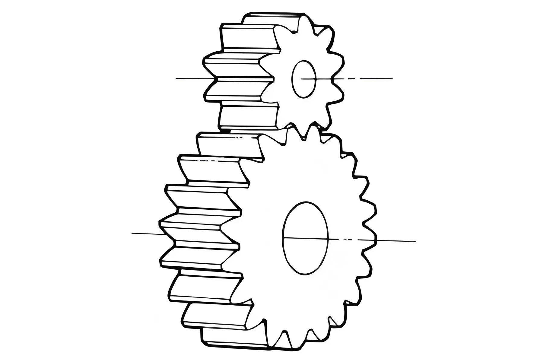
The pursuit of high-precision motion transmission is a fundamental objective in mechanical engineering, with the spur gear pair serving as one of the most ubiquitous and critical components. The performance of a spur gear transmission is traditionally evaluated based on criteria such as load capacity, efficiency, and noise. However, transmission accuracy, which quantifies the fidelity of angular motion transfer between the input and output shafts, is paramount for advanced applications in robotics, precision machine tools, and aerospace mechanisms. This accuracy is fundamentally compromised by the inherent imperfections within the transmission system, leading to a phenomenon known as time-varying center distance.
Classical gear theory often assumes ideal conditions: perfectly rigid components, geometrically perfect tooth profiles, and fixed, ideal support centers. In reality, a spur gear transmission system is an assembly of multiple components including shafts, gears, bearings, and housing. Each component introduces geometric errors from manufacturing and elastic deformations under operational loads. The bearings, which form the crucial interface between the rotating shafts and the static housing, are particularly significant. Their internal raceway errors (e.g., out-of-roundness like eccentricity, ellipticity, or lobing) and their compliance under radial loads cause the instantaneous centers of the supporting shafts to deviate from their nominal positions. This deviation is not static; it varies periodically with shaft rotation. Consequently, the actual distance between the centers of the mating spur gears fluctuates during operation. This time-varying center distance directly induces kinematic transmission error, exacerbates dynamic loads, and increases noise and vibration, ultimately degrading the overall transmission precision. Therefore, developing a comprehensive model that encapsulates the combined influence of support errors and elasticity is essential for accurate prediction, analysis, and design of high-precision spur gear drives.
Analysis of System Imperfections and Modeling Philosophy
The actual structure of a common spur gear transmission system typically involves two parallel shafts, each supported by a pair of bearings in a fixed configuration within a housing. The gears are mounted on these shafts, often with a rigid connection (e.g., press fit or key). The primary sources of center distance variation originate from the bearing-shaft assemblies.
1. Geometric Errors of Bearing Assemblies: The geometric inaccuracies of the bearing inner raceway are a primary source of support center movement. These errors are periodic in nature and can be represented by a Fourier series describing the deviation from a perfect circle. The radial error function of the inner raceway can be expressed as:
$$g_C(\theta) = r_0 + \sum_{n=1}^{\infty} E_n \cdot \sin(n \cdot \theta + \psi_n)$$
where $r_0$ is the nominal raceway radius, $\theta$ is the angular position, $E_n$ is the amplitude of the $n$-th harmonic error component, and $\psi_n$ is its corresponding phase angle. Common forms include:
– $n=1$: Eccentricity.
– $n=2$: Elliptical or oval shape.
– $n=3$: Triangular lobing (a common manufacturing artifact).
2. Elastic Deformation of Bearing Assemblies: Under the transmitted load, the entire bearing assembly (including the bearing itself, the shaft segment, and the housing) deforms elastically. This compliance allows the shaft center to shift radially under load. The relationship between the radial load on a bearing and the gear mesh force is given by static equilibrium. For a shaft with two supports and a gear placed between them, the radial bearing force $F_{Br}$ is:
$$F_{Br} = F_H \cdot \frac{L_a}{L}$$
where $F_H$ is the gear mesh force component, $L$ is the distance between bearing centers (span), and $L_a$ is the distance from the gear to the bearing in question.
The modeling challenge is to integrate these distributed, coupled errors and compliances into a tractable analytical framework. The core idea is to use the principle of kinematic equivalence. The physical bearing support with its combined geometric error and elasticity is conceptually replaced by an equivalent mechanism: a rigid cam profile representing the geometric error, whose follower is constrained by springs representing the elastic compliance. This transforms the complex support into a classic cam-follower system with elastic constraints.
Furthermore, applying the principle of relative motion, the errors and elasticities from both the input and output shafts can be consolidated into a single floating shaft model. One shaft (e.g., the output shaft) is considered ideally rigid and fixed in space. All geometric errors and elastic deformations from both shaft systems are then mapped onto the supports of the other shaft (the input shaft). This results in a model with a floating input shaft and a fixed ideal output shaft, which fully captures the relative center distance variation.
The Time-Varying Center Distance Model for Spur Gears
The proposed model for analyzing the spur gear transmission with time-varying center distance is constructed as follows. The input shaft, carrying the driving spur gear, is supported by two equivalent cam-follower mechanisms at its ends. Each cam corresponds to the equivalent geometric error of a bearing assembly on the floating shaft. Since the radial displacement has two degrees of freedom (along the X and Y axes in the gear plane), each cam is engaged by two pairs of opposed, spring-loaded translational followers. These followers act along the X and Y axes, creating a spring-constrained, conjugate cam-follower system. The springs are linear and only take compression, simulating the unilateral contact in bearings. The output shaft, carrying the driven spur gear, is modeled as perfectly rigid and ideally positioned.
Coordinate Systems: Defining coordinate systems is crucial for formulating the displacement equations.
– $S_f \{ O_f; X_f, Y_f, Z_f \}$: Fixed frame attached to the ideal center $O_f$ of the output spur gear. The $X_f$ axis aligns with the nominal centerline direction.
– $S_{C_i} \{ O_{C_i}; X_{C_i}, Y_{C_i}, Z_{C_i} \}$: Frame attached to the theoretical center $O_{C_i}$ of the $i$-th cam ($i=1,2$).
– $S_{ij}^{V} \{ O_{ij}; X_{ij}, Y_{ij}, Z_{ij} \}^{V}$: Frame attached to the $j$-th follower ($j=1,2$) in the $V$ direction ($V=X, Y$). The origin $O_{ij}^V$ represents the point of contact on the follower guide.
The cam profile, representing the mapped geometric error, is defined in its local frame $S_{C_i}$ by the polar equation $g_C(\theta)$ from Eq. (1). The instantaneous position of the floating cam center $O_{C_i}$ in the fixed frame $S_f$ is unknown a priori and must be solved from equilibrium conditions.
Equivalent Spring Stiffness: The stiffness $K_{ij}^V$ of each follower spring is not simply the bearing stiffness. It must represent the combined series compliance of the corresponding bearing assembly from both the floating input shaft and the fixed output shaft, mapped onto the single equivalent follower. If $K_{Br1j}^V$ and $K_{Br2j}^V$ are the actual bearing assembly stiffnesses in the $V$ direction for the input and output shafts, respectively, the equivalent follower stiffness is given by:
$$\frac{1}{K_{ij}^V} = \frac{1}{K_{Br1j}^V} + \frac{1}{K_{Br2j}^V}$$
The bearing assembly stiffness $K_{Br}^V$ itself is a combination of the rolling bearing stiffness $K_B$ and the supporting structure stiffness (shaft, housing) $K_{Sr}$, calculated as a spring in series:
$$\frac{1}{K_{Br}^V} = \frac{1}{K_B} + \frac{1}{K_{Sr}^V}$$
For a deep-groove ball bearing, the nonlinear stiffness $K_B$ can be approximated by a formula such as:
$$K_B = 32,375 \cdot N \cdot D_w^{1/2} \cdot \delta_r^{1/2} \cdot \cos^{5/2}\alpha_B$$
$$\cos\alpha_B = 1 – \frac{u_r}{2D_w(f_i + f_e – 1)}$$
where $N$ is the number of rolling elements, $D_w$ is the ball diameter, $\delta_r$ is the radial deformation, $\alpha_B$ is the contact angle, $u_r$ is the radial clearance, and $f_i$, $f_e$ are the inner and outer raceway curvature coefficients.
Fundamental Equations for System Solution
For a given input rotation angle $\phi_1$, the position of the floating input shaft center (and thus the driving spur gear center) is determined by solving a set of geometric compatibility and static equilibrium equations.
1. Displacement Compatibility Equations: Considering one equivalent cam-follower mechanism, the vector loop equation for contact in the $V$ direction is:
$$\mathbf{r}_{OC_i} + \mathbf{r}_{ij}^V + (L_{ij}^V – \delta_{ij}^V) = L_{Dj}/2$$
Here, $\mathbf{r}_{OC_i}$ is the position vector of cam center $O_{C_i}$ in $S_f$. $\mathbf{r}_{ij}^V$ is the vector from $O_{C_i}$ to the cam contact point $P_{ij}^{Vf}$. $L_{ij}^V$ is the fixed position vector of the follower guide axis. $\delta_{ij}^V$ is the elastic compression of the follower spring. $L_{Dj}/2$ is a constant locating the follower guide relative to the fixed frame origin $O_f$.
Expanding this for two cams ($i=1,2$), two directions ($V=X,Y$), and two followers per direction ($j=1,2$), yields 8 scalar displacement equations. The unknowns in these equations include the 4 coordinates defining the two cam center positions $\mathbf{r}_{OC_1}=(x_1, y_1)$, $\mathbf{r}_{OC_2}=(x_2, y_2)$ and the 8 spring compressions $\delta_{ij}^V$, totaling 12 unknowns at this stage.
2. Static Equilibrium Equations:
a) Force Balance for the Floating Input Shaft: The input shaft is subjected to contact forces $\mathbf{F}_{ij}^V$ from the cam followers and the gear mesh force $\mathbf{F}_H$. Force equilibrium requires:
$$\sum_{i=1}^{2}\sum_{j=1}^{2} (\mathbf{F}_{ij}^X + \mathbf{F}_{ij}^Y) + \mathbf{F}_H = 0$$
This provides 2 scalar equations (in the X and Y directions), introducing 8 new unknowns: the magnitudes of the cam contact forces $F_{ij}^V$.
b) Force Balance for Individual Followers: For each spring-loaded follower, equilibrium in the direction of motion relates the cam contact force $F_{ij}^V$, the spring force $F_{ij}^{VK}$, and the guide reaction force $F_{ij}^{Vf}$. The spring force is related to the cam force by the pressure angle $\alpha_{ij}^V$ at the contact point:
$$F_{ij}^{VK} = F_{ij}^V \cos\alpha_{ij}^V$$
$$F_{ij}^{Vf} = F_{ij}^{VK} \tan\alpha_{ij}^V$$
The spring force is linearly related to its compression (for small deformations):
$$F_{ij}^{VK} = K_{ij}^V \cdot \delta_{ij}^V$$
These provide 8 additional equations without introducing new variables.
c) Force and Moment Balance for the Output Shaft: The output shaft is subject to bearing reaction forces $\mathbf{F}_{Bj}^V$ (which are the mapped counterparts of the input shaft’s bearing loads) and the output torque $T_O$. Equilibrium gives:
$$\sum (\mathbf{F}_{Bj}^V) + \mathbf{F}_H = 0$$
$$F_H \cdot r_{b2} + T_O = 0$$
where $r_{b2}$ is the base circle radius of the driven spur gear, and $F_H$ is the magnitude of the mesh force. This provides 3 scalar equations (2 force, 1 moment), introducing the mesh force magnitude $F_H$ and the output torque $T_O$ as solvable parameters given the input torque $T_I$.
In summary, the complete system consists of:
– 8 Displacement equations.
– 2 Input shaft force equilibrium equations.
– 8 Follower equilibrium/spring force equations.
– 3 Output shaft equilibrium equations.
This gives a total of 21 equations. The primary unknowns are: 4 cam center coordinates ($x_1, y_1, x_2, y_2$), 8 spring compressions ($\delta_{ij}^V$), and 8 cam contact forces ($F_{ij}^V$), plus the mesh force $F_H$ — totaling 21 unknowns. The system is therefore solvable numerically for each input angle $\phi_1$.
Derivation of the Time-Varying Center Distance Function
Once the cam center positions $\mathbf{r}_{OC_1}$ and $\mathbf{r}_{OC_2}$ are solved for a given input angle $\phi_1$, the actual position of the driving spur gear center $O_1$ in the fixed frame $S_f$ is found. Assuming the gear is rigidly connected to the shaft, its center is the midpoint of the line connecting the two equivalent support centers (cam centers):
$$\mathbf{r}_{O_1}^{f} = \frac{\mathbf{r}_{OC_1} + \mathbf{r}_{OC_2}}{2}$$
This point $\mathbf{r}_{O_1}^{f}$ represents the trajectory of the gear center relative to the fixed output gear center $O_f$. The instantaneous center distance $a(\phi_1)$ is the magnitude of the vector from $O_f$ to $O_1$. However, to express it in the conventional sense (distance from input to output gear center), we note that in the model, $O_f$ is fixed at the nominal output gear center. The vector $\mathbf{r}_{O_1}^{f}$ itself gives the deviation of the input gear center. The actual center distance is therefore the distance between $O_1$ and the fixed point $O_f$, which is simply $||\mathbf{r}_{O_1}^{f}||$. More informatively, we can define the center distance error $\Delta a(\phi_1)$ as the deviation from the nominal center distance $a_0$:
$$\Delta a(\phi_1) = ||\mathbf{r}_{O_1}^{f}|| – a_0$$
Alternatively, since the primary relative motion is along the line of centers ($X_f$ direction), the component $r_{O_1, X}^{f}$ often dominates. The function $\Delta a(\phi_1)$ is periodic with the rotation of the input shaft and encapsulates the combined effects of bearing geometric errors, system elasticity, and applied load.
Case Study: Influence of Parameters on Center Distance Variation
To illustrate the application and insights gained from the model, consider a specific spur gear transmission example. The nominal operating conditions and key parameters are listed below.
| Parameter | Symbol | Value | Unit |
|---|---|---|---|
| Input Torque | $T_I$ | 47 | Nm |
| Module | $m$ | 4 | mm |
| Number of Teeth (Driver) | $z_1$ | 20 | – |
| Number of Teeth (Driven) | $z_2$ | 25 | – |
| Nominal Center Distance | $a_0$ | 90 | mm |
| Shaft Diameter | $D$ | 30 | mm |
| Bearing Span | $L$ | 200 | mm |
| Gear Location from Bearing | $L_a$ | 100 | mm |
| Shaft Young’s Modulus | $E$ | 2.05e5 | MPa |
| Shaft Shear Modulus | $G$ | 80e3 | MPa |
The bearings are P0 grade 6006 deep-groove ball bearings. Their internal geometry and the calculated/mapped equivalent model parameters are as follows.
| Parameter | Value | Unit |
|---|---|---|
| Bearing Inner Diameter, $d$ | 30 | mm |
| Bearing Outer Diameter, $D$ | 55 | mm |
| Ball Diameter, $D_w$ | 7.144 | mm |
| Number of Balls, $N$ | 11 | – |
| Inner Raceway Curvature Coeff., $f_i$ | 0.515 | – |
| Outer Raceway Curvature Coeff., $f_e$ | 0.525 | – |
| Initial Radial Clearance, $u_r$ | 0.018 | mm |
| Nominal Raceway Radius, $r_0$ | 17.678 | mm |
| Equivalent Follower Guide Distance, $L_{Dj}/2$ | 24.822 | mm |
| Equivalent Follower Stiffness (Avg.), $K_{ij}^V$ | ~3.5e5 | N/mm |
The bearing geometric error is assumed to be dominated by a triangular lobing shape ($n=3$ in Eq. (1)). We investigate the effect of three key factors on the time-varying center distance error $\Delta a(\phi_1)$.
1. Effect of Load Magnitude: The input torque is varied as $T_I = 9.4, 23.5,$ and $47 \text{ Nm}$. The error amplitude $E_3$ is held constant at $5 \mu m$, and the phase $\psi$ is zero. The results show that increasing the load primarily scales the amplitude of the center distance variation. The waveform shape, dictated by the third harmonic error, remains largely unchanged. This indicates that the elastic deformation under load acts as a linear amplification factor superimposed on the geometric error-induced motion. The relationship between load and center distance fluctuation amplitude is nonlinear due to the nonlinear bearing stiffness but is monotonic.
2. Effect of Geometric Error Amplitude: The amplitude of the third harmonic $E_3$ is varied as $2.5, 5.0,$ and $10.0 \mu m$, while the input torque is kept at the nominal $47 \text{ Nm}$ and phase $\psi=0$. Unsurprisingly, a larger geometric error directly produces a larger center distance variation. The waveform shape is again preserved, confirming that the geometric error profile is the primary driver of the variation pattern. The elastic deformation modifies the magnitude but not the fundamental harmonic content originating from the cam profile.
3. Effect of Geometric Error Phase: This is a critical and less obvious factor. The model incorporates two cams (one at each support). The phase difference $\Delta\psi$ between the geometric errors at these two supports significantly affects the resulting motion of the spur gear center. Let the phase of the error on the two supports be $\psi_1$ and $\psi_2$. We examine cases where $\Delta\psi = \psi_2 – \psi_1 = \pi/4, \pi/3, \pi/2$, with $E_3=5 \mu m$ and $T_I=47 \text{ Nm}$.
– When the phase difference is small or zero, the motions from both supports add constructively along certain directions, leading to a larger resultant center distance error.
– As the phase difference increases, the motions can partially cancel each other, especially the lateral (Y-direction) components, leading to a different trajectory for the gear center $O_1$. The $\Delta a(\phi_1)$ curve changes not only in amplitude but also in its shape.
– In the specific cases analyzed, a phase difference of $\pi/4$ resulted in the smallest peak-to-peak variation in $\Delta a(\phi_1)$. This finding is significant for precision assembly, suggesting that intentionally controlling or selecting the angular orientation (phasing) of bearings during assembly could be a practical method to minimize transmission error in a spur gear system, even without improving the individual bearing quality.
Conclusion
This analysis establishes a comprehensive framework for modeling and understanding the time-varying center distance in spur gear transmissions. By integrating the geometric errors and elastic compliances of bearing assemblies into a unified cam-follower equivalent model, we move beyond the analysis of the gear pair in isolation. The derived system of equations allows for the numerical determination of the instantaneous gear center position under load, from which the critical center distance variation function $\Delta a(\phi_1)$ is obtained.
The key insights from the model and case study are:
1. The time-varying center distance is an inherent characteristic of real spur gear systems, arising from the synergy of component errors and system elasticity.
2. The pattern of variation is primarily dictated by the harmonic content of the bearing raceway geometric errors.
3. The magnitude of the variation is linearly amplified by both the amplitude of these geometric errors and the applied load (via nonlinear system compliance).
4. The relative phase of geometric errors at different support locations is a crucial factor. Optimal phasing can significantly reduce the resultant center distance variation, providing a viable strategy for enhancing the accuracy of spur gear transmissions through precision assembly, even with components of finite individual accuracy.
This model provides a foundational theoretical tool for the accuracy analysis and design of precision gear drive systems. It creates a direct link between the manufacturing quality of components (like bearings), the system’s structural design (stiffness), operational conditions (load), and the final kinematic performance of the spur gear transmission. Future work can extend this model to include gear tooth flexibility, more complex system dynamics, and the optimization of support parameters for minimal transmission error.