
In the field of aerospace engineering, the demand for high-performance gear transmission systems is ever-increasing, particularly in applications such as aero-engine gearboxes. Among various gear types, the herringbone gear has garnered significant attention due to its unique ability to cancel axial thrust forces, making it ideal for high-speed and high-load scenarios. My research focuses on the dynamics modeling and analysis of a split torque transmission system incorporating herringbone gears, which is critical for ensuring reliability and efficiency in aviation power transmission. This work delves into the complexities of such systems, considering factors like time-varying mesh stiffness, static transmission errors, bearing supports, and gyroscopic effects. The primary goal is to develop a robust computational framework that can accurately predict dynamic behaviors, thereby aiding in the design and optimization of herringbone gear systems for aerospace applications.
The study begins with an overview of gear dynamics, where internal and external excitations play pivotal roles. Internal excitations include time-varying mesh stiffness, static and dynamic transmission errors, tooth profile modifications, and backlash, while external excitations encompass input torque fluctuations and rotational speed variations. For herringbone gears, which consist of two helical gears with opposite hand angles, the dynamics are further complicated by interactions between the left and right helical segments. Traditional modeling approaches often simplify these aspects, but in this research, I aim to incorporate detailed considerations to enhance accuracy. The finite element node method is employed, leveraging Timoshenko beam theory to model shafts and rotor dynamics, allowing for a comprehensive analysis of system modes and responses.
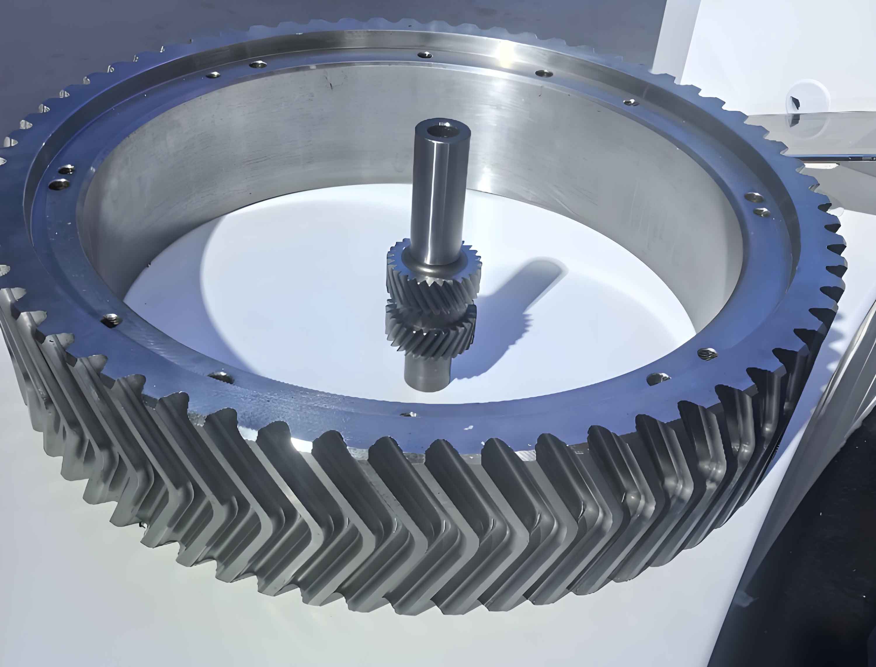
To set the stage, let’s consider the split torque transmission system used in an aero-engine gearbox. This system features an input herringbone gear meshing with two first-stage driven herringbone gears, which are connected via shafts to second-stage driving herringbone gears. These, in turn, mesh with a second-stage driven herringbone gear coupled to the output shaft. The herringbone gear design is essential here, as it mitigates axial loads and improves load distribution. The basic parameters of the herringbone gear train are summarized in the table below, which includes key dimensions such as tooth numbers, module, pressure angle, helix angle, and face width. These parameters form the foundation for the dynamic model.
| Parameter | Input Gear | First-Stage Driven Gear | Second-Stage Driving Gear | Second-Stage Driven Gear |
|---|---|---|---|---|
| Number of Teeth | 29 | 113 | 26 | 125 |
| Module (mm) | 2.75 | 2.75 | 4.25 | 4.25 |
| Pressure Angle (°) | 25 | 25 | 25 | 25 |
| Helix Angle (°) | 30 | 30 | 30 | 30 |
| Face Width (mm) | 65 | 65 | 85 | 85 |
| Tooth Space Width (mm) | 25 | 25 | 30 | 30 |
The dynamics model is constructed using the finite element node method, where each component—gears, shafts, and bearings—is discretized into nodes connected by elements. For the herringbone gear rotors, the kinetic energy includes both translational and rotational components, leading to equations of motion that account for gyroscopic effects. The angular velocity of a gear rotor can be expressed as:
$$ \omega_i = \left[ \cos(\Omega_i + \dot{\theta}_{zi}) \dot{\theta}_{yi} + \sin(\Omega_i + \dot{\theta}_{zi}) \dot{\theta}_{xi} \right] \mathbf{i} + \left[ \sin(\Omega_i + \dot{\theta}_{zi}) \dot{\theta}_{yi} – \cos(\Omega_i + \dot{\theta}_{zi}) \dot{\theta}_{xi} \right] \mathbf{j} + \left[ (\Omega_i + \dot{\theta}_{zi}) + \frac{\theta_{xi} \dot{\theta}_{yi} – \theta_{yi} \dot{\theta}_{xi}}{2} \right] \mathbf{k} $$
where \( \Omega_i \) is the rotational speed, and \( \theta_{xi}, \theta_{yi}, \theta_{zi} \) are angular displacements about the X, Y, and Z axes, respectively. Applying Lagrange’s equations, the motion equation for a gear rotor is derived as:
$$ [M^d_i] \ddot{\mathbf{q}}_i + \Omega_i [G^d_i] \dot{\mathbf{q}}_i = \mathbf{F}^d_i $$
Here, \( [M^d_i] \) is the mass matrix, \( [G^d_i] \) is the gyroscopic matrix, and \( \mathbf{q}_i = [x_i, y_i, z_i, \theta_{xi}, \theta_{yi}, \theta_{zi}]^T \) represents the displacement vector. The mass matrix is diagonal: \( M^d_i = \text{diag}(m_i, m_i, m_i, J_{Di}, J_{Di}, J_{Pi}) \), with \( m_i \) as mass, \( J_{Di} \) as diametral moment of inertia, and \( J_{Pi} \) as polar moment of inertia. The gyroscopic matrix captures the coupling due to rotation:
$$ G^d_i = \begin{bmatrix}
0 & 0 & 0 & 0 & 0 & 0 \\
0 & 0 & 0 & 0 & 0 & 0 \\
0 & 0 & 0 & 0 & 0 & 0 \\
0 & 0 & 0 & 0 & J_{Pi} & 0 \\
0 & 0 & 0 & -J_{Pi} & 0 & 0 \\
0 & 0 & 0 & 0 & 0 & 0
\end{bmatrix} $$
For the meshing action of herringbone gears, each helical pair is modeled separately, considering the opposite helix angles. The relative displacement along the line of action for a single helical pair is given by:
$$ \delta_m = \left[ (x_p – x_g) \sin \phi + (y_p – y_g) \cos \phi + (r_p \theta_{pz} + r_g \theta_{gz}) \right] \cos \beta + \left[ (r_p \theta_{py} + r_g \theta_{gy}) \cos \phi + (r_p \theta_{px} + r_g \theta_{gx}) \sin \phi + (z_g – z_p) \right] \sin \beta – e_{ste}(t) $$
where \( \phi \) is the pressure angle, \( \beta \) is the helix angle, \( r_j \) is the base circle radius, and \( e_{ste}(t) \) is the static transmission error. The meshing force on the normal line includes stiffness, damping, and backlash effects:
$$ F_m = k_m (\gamma_{m0} \delta_m + \gamma_{m1} B) + c_m \gamma_{m0} \dot{\delta}_m $$
The functions \( \gamma_{m0} \) and \( \gamma_{m1} \) handle backlash: \( \gamma_{m0} = 1 \) if \( |\delta_m| > B \), else 0; \( \gamma_{m1} = -1 \) if \( \delta_m > B \), 1 if \( \delta_m < -B \), else 0. Here, \( B \) is the backlash, \( k_m \) is the time-varying mesh stiffness, and \( c_m \) is the damping coefficient. This nonlinear formulation is crucial for capturing realistic herringbone gear dynamics. The mesh stiffness \( k_m \) varies periodically with engagement, and for herringbone gears, it can be expressed as a Fourier series:
$$ k_m(t) = k_{hm} + \sum_{r=1}^{\infty} k_{hr} \cos(r \omega_h t) $$
where \( k_{hm} \) is the average mesh stiffness, \( k_{hr} \) are harmonic amplitudes, and \( \omega_h \) is the mesh frequency. To compute this, finite element analysis is performed on herringbone gear pairs, meshing teeth with hexahedral elements and applying loads at reference points. The results show that the mesh stiffness for herringbone gears fluctuates cyclically, with significant variations at tooth entry and exit points due to deformation and impact.
Shafts are modeled using Timoshenko beam elements, which account for bending, shear, and torsion. Each beam element has four degrees of freedom per node: translations in X and Y directions, and rotations about X and Y axes. The equation of motion for a shaft element is:
$$ M^e \ddot{\mathbf{q}}_e + \Omega G^e \dot{\mathbf{q}}_e + K^e \mathbf{q}_e = 0 $$
where \( M^e \), \( G^e \), and \( K^e \) are the element mass, gyroscopic, and stiffness matrices, respectively. Assembling all elements gives the global shaft dynamics. Bearings are simplified as spring-damper systems with stiffness and damping matrices. For angular contact ball bearings used in herringbone gear systems, the stiffness matrix is:
$$ K_B = \begin{bmatrix}
k_{xx} & k_{xy} & k_{xz} & k_{x\theta_x} & k_{x\theta_y} & k_{x\theta_z} \\
k_{yx} & k_{yy} & k_{yz} & k_{y\theta_x} & k_{y\theta_y} & k_{y\theta_z} \\
k_{zx} & k_{zy} & k_{zz} & k_{z\theta_x} & k_{z\theta_y} & k_{z\theta_z} \\
k_{\theta_x x} & k_{\theta_x y} & k_{\theta_x z} & k_{\theta_x \theta_x} & k_{\theta_x \theta_y} & k_{\theta_x \theta_z} \\
k_{\theta_y x} & k_{\theta_y y} & k_{\theta_y z} & k_{\theta_y \theta_x} & k_{\theta_y \theta_y} & k_{\theta_y \theta_z} \\
k_{\theta_z x} & k_{\theta_z y} & k_{\theta_z z} & k_{\theta_z \theta_x} & k_{\theta_z \theta_y} & k_{\theta_z \theta_z}
\end{bmatrix} $$
In practice, coupling terms are often neglected, so the matrix simplifies to diagonal entries for radial, axial, and angular stiffness. Damping is modeled proportionally: \( C = \alpha M + \beta K \), where \( \alpha \) and \( \beta \) are coefficients determined empirically.
Combining all components, the global nonlinear dynamics equation for the herringbone gear split torque transmission system is:
$$ M \ddot{\mathbf{q}} + (C + \Omega G) \dot{\mathbf{q}} + K f(\mathbf{q}) = \mathbf{F}(t) $$
Here, \( M \), \( C \), \( G \), and \( K \) are the global mass, damping, gyroscopic, and stiffness matrices; \( f(\mathbf{q}) \) is a nonlinear function representing backlash; and \( \mathbf{F}(t) \) includes external loads and internal excitations like static transmission errors. This equation forms the basis for modal and response analyses.
Next, I compute the natural frequencies of the system using vibration theory methods. The finite element node model, with Timoshenko beams, efficiently captures bending, axial, and torsional modes. The table below lists the natural frequencies up to 5000 Hz, which are essential for identifying resonance risks in herringbone gear operation.
| Mode Order | Frequency (Hz) | Mode Order | Frequency (Hz) |
|---|---|---|---|
| 1 | 27.1 | 13 | 1194.1 |
| 2 | 97.8 | 14 | 1452.3 |
| 3 | 138.5 | 15 | 1818 |
| 4 | 142.3 | 16 | 2003 |
| 5 | 285.1 | 17 | 2262 |
| 6 | 368.7 | 18 | 2414 |
| 7 | 559.6 | 19 | 2881 |
| 8 | 624.9 | 20 | 3213 |
| 9 | 695.8 | 21 | 3896 |
| 10 | 838.5 | 22 | 4410 |
| 11 | 897.4 | 23 | 4657 |
| 12 | 1023 | 24 | 4957.3 |
The frequencies are dense in the low range, which could be easily excited by imbalances or loosened components. Notably, frequencies around 1818 Hz and 4410 Hz correspond to the second-stage and first-stage herringbone gear mesh frequencies, respectively, posing potential vibration issues. To delve deeper, I analyze mode shapes at key frequencies: 368.7 Hz, 838.5 Hz, 1818 Hz, and 4410 Hz. At 368.7 Hz, the mode shape shows significant disparities between the two branches of the herringbone gear train, indicating possible load imbalance. At higher frequencies like 1818 Hz, the second-stage driven herringbone gear exhibits large amplitudes, which could lead to excessive vibrations if excited. These insights are critical for design improvements.
Experimental validation is conducted on a gearbox test rig, with accelerometers placed on the housing near bearings. The measured natural frequencies align well with simulations, as shown in the comparison table below. The errors are within 7%, confirming the model’s accuracy for herringbone gear applications.
| Experimental Frequency (Hz) | Simulated Frequency (Hz) | Error |
|---|---|---|
| 361 | 368.7 | 2.1% |
| 834 | 838.5 | 0.5% |
| 1818 | 1818 | 0% |
| 4415 | 4410 | 0.1% |
For dynamic response analysis, I calculate the time-varying mesh stiffness and static transmission error specifically for herringbone gears. Using finite element methods, the mesh stiffness of a second-stage herringbone gear pair is computed under loaded conditions. The stiffness curve exhibits periodic fluctuations, with an average value of approximately \( 1.2 \times 10^9 \, \text{N/m} \). The Fourier decomposition reveals harmonic components that contribute to dynamic excitations. The static transmission error is derived from measured tooth surface data, following a process that involves coordinate extraction, error superposition, and envelope fitting. For herringbone gears, the left and right helical pairs may have different errors, but axial floating designs in the system help mitigate these disparities. The static transmission error is predominantly low-frequency, with amplitudes decaying at higher orders, as summarized in the table below for a herringbone gear pair.
| Harmonic Order | Amplitude (μm) | Frequency Component |
|---|---|---|
| 1 | 5.2 | Fundamental |
| 2 | 3.1 | 2nd Harmonic |
| 3 | 1.8 | 3rd Harmonic |
| 4 | 0.9 | 4th Harmonic |
| 5 | 0.4 | 5th Harmonic |
With these inputs, I solve the nonlinear dynamics equation using the Newmark-beta method, a numerical integration technique suitable for transient analysis. The time-domain response is simulated at a node near the output bearing, where vibrations are transmitted to the housing. The acceleration signals show convergence and modulation phenomena, indicative of beating between different frequency components. For instance, at an input speed of 16,350 rpm and power of 2,500 kW, the simulated acceleration exhibits peaks due to impacts from backlash and mesh stiffness variations. Comparing with experimental data, both show similar trends, though experimental signals are smoother due to damping from the housing and parameter uncertainties in the model. The frequency-domain responses, obtained via Fast Fourier Transform (FFT), highlight key spectral components. The table below compares dominant frequencies in simulation and experiment for the herringbone gear system.
| Frequency Type | Simulated Value (Hz) | Experimental Value (Hz) | Remarks |
|---|---|---|---|
| 2nd-Stage Mesh Frequency | 1818 | 1818 | Primary excitation |
| 1st-Stage Mesh Frequency | 4410 | 4415 | Sub-harmonic observed |
| Shaft Frequency Harmonics | 97.8, 285.1 | ~100, ~290 | Due to unbalance |
| Combination Frequencies | 4883, 5356 | ~4900, ~5360 | Coupling of mesh and shaft tones |
The spectrum reveals not only mesh frequencies and their multiples but also sidebands and combination tones, such as 4883 Hz and 5356 Hz, which arise from interactions between herringbone gear meshing and shaft rotations. In experiments, resonance bands appear around 1818 Hz, attributed to external random excitations not modeled in simulations. This underscores the complexity of herringbone gear dynamics in real-world conditions.
To further elaborate on herringbone gear modeling, I consider the effects of asymmetric errors between left and right helices. These errors can alter load distribution and dynamic transmission errors, but in split torque systems, they are often compensated by flexible couplings or floating elements. The equations for meshing forces are extended to include separate terms for each helix, enhancing the model’s fidelity. For instance, the relative displacement for the left helix of a herringbone gear pair is modified by incorporating specific error profiles, leading to refined excitation functions.
In terms of damping, proportional damping is assumed, but for herringbone gears, material hysteresis and oil film effects in bearings may introduce nonlinearities. Future models could integrate velocity-dependent damping matrices based on empirical data. Additionally, the gyroscopic matrix \( G \) plays a significant role at high speeds, causing frequency splits and mode shape changes, which are critical for herringbone gear rotors due to their large polar moments of inertia.
The advantages of the finite element node method for herringbone gear systems are manifold. It efficiently handles complex geometries, allows for parameter studies (e.g., varying helix angles or backlash), and facilitates integration with control systems for active vibration suppression. For example, adjusting the helix angle of herringbone gears from 30° to 25° could reduce axial forces but alter mesh stiffness, impacting dynamics—a trade-off easily explored with this model.
In conclusion, my research on herringbone gear split torque transmission systems demonstrates the efficacy of finite element node-based dynamics modeling. The approach accurately predicts natural frequencies, mode shapes, and dynamic responses, validated against experimental data. Key findings include the identification of critical frequencies that correlate with herringbone gear meshing, the importance of considering backlash and time-varying stiffness, and the presence of modulation effects in time-domain signals. This methodology offers valuable insights for designing robust herringbone gear systems in aerospace applications, where reliability and performance are paramount. Future work could focus on incorporating thermal effects, wear progression, and advanced damping models to further enhance the predictive capability for herringbone gear dynamics.