
In modern marine propulsion systems, herringbone gears are extensively employed due to their superior load-carrying capacity, ability to cancel axial thrust forces, and smooth operational characteristics. As a researcher focused on gear dynamics, I have dedicated significant effort to understanding and improving the fatigue performance of these critical components. The complex and variable operating conditions of marine transmissions, including sudden load changes and high torque demands, necessitate a thorough investigation into the dynamic behavior of herringbone gears, particularly the fluctuating stresses at the tooth root, which are a primary precursor to bending fatigue failure. This article presents a comprehensive methodology I developed to predict the bending fatigue life of herringbone gear teeth based on dynamic root stress analysis and proposes an effective three-dimensional tooth surface modification strategy to extend service life.
The fundamental mechanism behind tooth bending fatigue failure lies in the alternating tensile stresses experienced at the tooth root fillet on the loaded side. While compressive stresses also exist, it is the tensile stress concentration that predominantly drives crack initiation and propagation. To accurately capture these dynamic tensile stresses, I established a sophisticated twelve-degree-of-freedom (12-DOF) coupled bending-torsion-axial vibration model for a herringbone gear pair. This model meticulously incorporates key dynamic excitations: time-varying mesh stiffness, transmission error-induced impacts, and friction forces at the tooth contact interfaces. The equations of motion for this system are derived from Lagrange’s equations and can be summarized in matrix form:
$$
\mathbf{M}\ddot{\mathbf{X}} + \mathbf{C}\dot{\mathbf{X}} + \mathbf{K}(t)\mathbf{X} = \mathbf{F}_{\text{m}}(t) + \mathbf{F}_{\text{error}}(t) + \mathbf{F}_{\text{fric}}(t)
$$
where $\mathbf{M}$, $\mathbf{C}$, and $\mathbf{K}(t)$ are the mass, damping, and time-varying stiffness matrices, respectively. $\mathbf{X}$ is the displacement vector containing the translational and rotational degrees of freedom for both the pinion and gear. The forcing vectors $\mathbf{F}_{\text{m}}(t)$, $\mathbf{F}_{\text{error}}(t)$, and $\mathbf{F}_{\text{fric}}(t)$ represent the forces due to static load transmission, manufacturing errors, and tooth surface friction. Solving this system dynamically provides the instantaneous dynamic mesh forces $F_{v,i}$ for each contacting tooth pair at every discrete time step $i$.
A critical aspect often overlooked in simplified analyses is the stress interaction between simultaneously engaged tooth pairs. When a particular tooth is not yet in direct contact, it can experience compressive root bending stresses due to the load borne by adjacent teeth. This pre-load compression phase subsequently influences the tensile stress cycle when that tooth enters the main load-bearing zone. My model accounts for this by superimposing the stress contributions from all active tooth pairs. The dynamic tensile stress $\sigma_{v,i}$ at the midpoint of the tooth root fillet on the tension side for the subject tooth at step $i$ is calculated as:
$$
\sigma_{v,i} = \sigma_{e,li} \cdot F_{v,i} – \sigma_{vy,i}
$$
Here, $\sigma_{e,li}$ is the static tensile stress at the root midpoint produced by a unit load, obtained through a detailed Loaded Tooth Contact Analysis (LTCA) that considers the three-dimensional contact ellipse and gear body compliance. $F_{v,i}$ is the dynamic load share on that tooth pair from the vibration model, and $\sigma_{vy,i}$ is the compressive stress induced at the same root point by the loading of neighboring teeth. The LTCA solves the compatibility equation for deformation under load:
$$
\mathbf{p} + \mathbf{w} = \mathbf{Z} + \mathbf{F} \cdot \mathbf{d}
$$
where $\mathbf{p}$ is the vector of discrete contact loads, $\mathbf{w}$ is the initial separation, $\mathbf{Z}$ is the rigid body approach, $\mathbf{F}$ is the flexibility matrix, and $\mathbf{d}$ is the deformed gap.
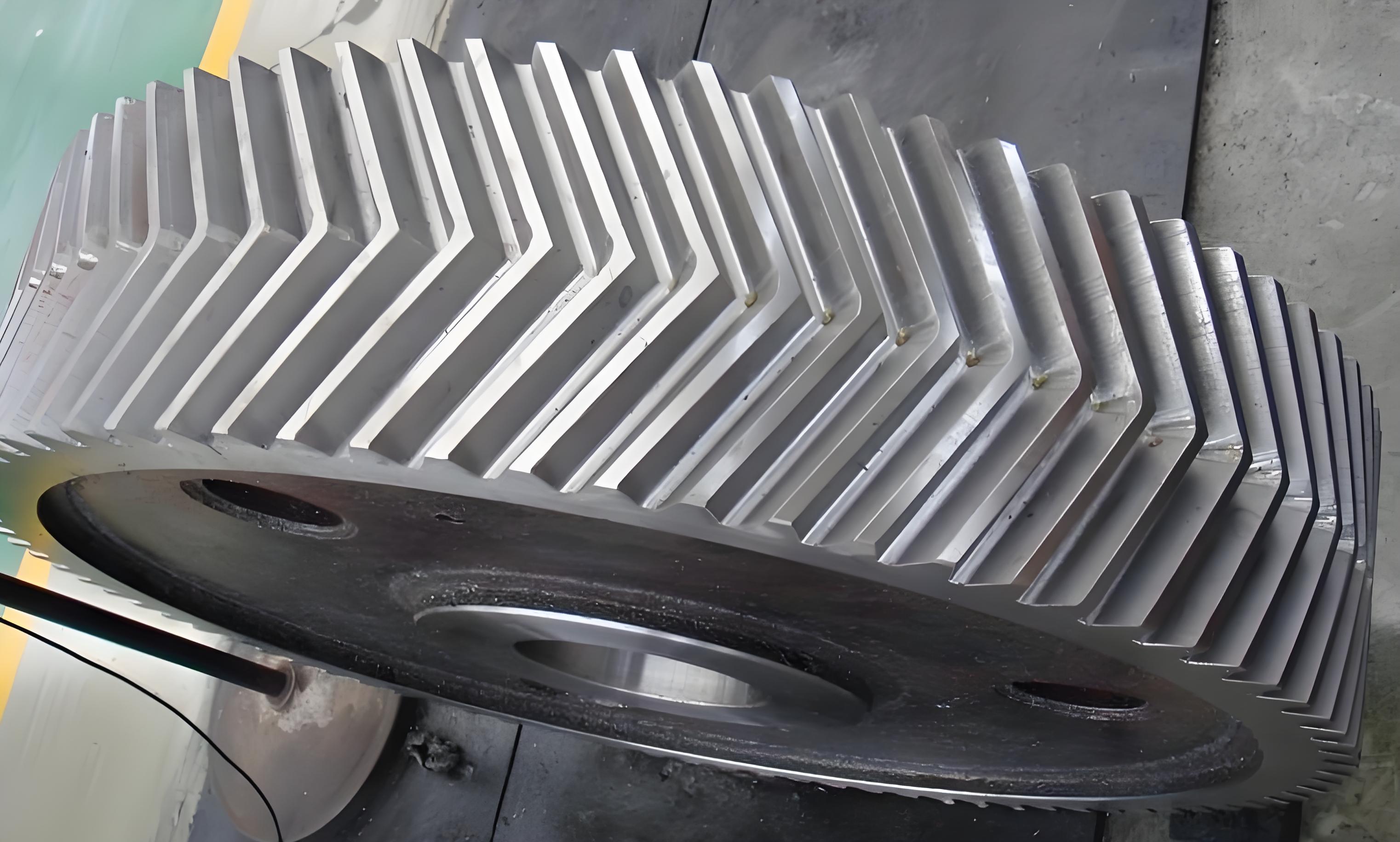
To demonstrate the application, I analyzed a marine single-stage herringbone gear set. The geometric and operational parameters are summarized in the table below. Marine systems often operate across a wide load spectrum; therefore, I considered three primary torque conditions: 50% (2000 Nm), 100% (4000 Nm), and 150% (6000 Nm) of the rated load.
| Parameter | Pinion (Driving) | Gear (Driven) |
|---|---|---|
| Normal Module (mm) | 6 | |
| Normal Pressure Angle (°) | 20 | |
| Helix Angle (°) | 24.43 (Left & Right Hand) | 24.43 (Right & Left Hand) |
| Number of Teeth | 17 | 44 |
| Face Width per Helix (mm) | 55 | 55 |
| Pinion Speed (rpm) | 2000 | – |
| Rated Torque (Nm) | 4000 | |
| Material | Quenched and Tempered Steel (Equivalent to AISI 1045) | |
| Density (g/cm³) | 7.85 | |
| Young’s Modulus (GPa) | 210 | |
The dynamic simulation yielded the time-history of the tensile root stress for the pinion under the three load cases. The results clearly showed the characteristic stress pattern: a compressive phase before the tooth enters the primary contact zone, followed by a sharp rise to a peak tensile stress, and then a decay. As expected, both the mean stress and the stress amplitude increased with higher applied torque. The fluctuating nature of this stress signal, with varying mean and amplitude, is a classic case for fatigue analysis using the stress-life (S-N) approach.
To predict the bending fatigue life, I processed the complex dynamic stress history using the rainflow counting algorithm. This method identifies all closed hysteresis loops (stress cycles) in the data, characterizing each cycle by its stress range ($\Delta \sigma$) and mean stress ($\sigma_m$). For non-zero mean stress cycles, I used the Goodman relation to convert them to equivalent fully reversed (zero mean) stress amplitudes ($\sigma_{a,eq}$) for comparison with the material’s S-N curve:
$$
\sigma_{a,eq} = \frac{\sigma_a}{1 – \frac{\sigma_m}{\sigma_u}}
$$
where $\sigma_a$ is the original stress amplitude, $\sigma_m$ is the original mean stress, and $\sigma_u$ is the ultimate tensile strength of the material (approximately 650 MPa for the gear steel). The material’s P-S-N curve, defining the stress-life relationship for a required reliability (99.9% in this marine application), is expressed as:
$$
\log_{10}(N) = a_p + b_p \cdot \log_{10}(\sigma_{a,eq})
$$
where $a_p$ and $b_p$ are material constants for the desired survival probability $p$. For the high-reliability case, I used $a_p = 26.3380$ and $b_p = -7.0415$. The fatigue damage for each stress cycle is calculated as $1/N$, where $N$ is the life in cycles corresponding to its $\sigma_{a,eq}$. According to Miner’s linear cumulative damage rule, failure is predicted when the sum of the damage fractions reaches unity. Therefore, the total life $L$ in number of stress blocks (one block representing the simulated time history) is:
$$
L = \frac{1}{\sum_{i} \frac{n_i}{N_i}}
$$
where $n_i$ is the number of cycles counted at a specific equivalent stress level, and $N_i$ is the fatigue life at that level from the S-N curve. For a combined duty cycle where the gear operates at different load levels for given fractions of time, the overall life is calculated as:
$$
\frac{1}{L_{\text{total}}} = \sum_{k=1}^{3} \frac{\chi_k}{L_k}
$$
Here, $\chi_k$ is the fraction of total operating time spent at load condition $k$ (I assumed $\chi = [0.2, 0.5, 0.3]$ for the 2000, 4000, and 6000 Nm cases, respectively), and $L_k$ is the calculated life if operated solely at that condition.
| Stress Range (MPa) | Mean Stress (MPa) | Equivalent Stress (MPa) | Cycles per Block (n_i) | Fatigue Life N_i (Cycles) | Damage per Block (n_i/N_i) |
|---|---|---|---|---|---|
| 15.2 | -5.1 | 15.0 | 2 | 1.2e10 | 1.67e-10 |
| 42.8 | 10.5 | 43.7 | 1 | 5.6e8 | 1.79e-9 |
| 68.5 | 25.8 | 72.1 | 1 | 8.9e7 | 1.12e-8 |
| … | … | … | … | … | … |
| Total Damage per Block | 4.85e-8 | ||||
| Predicted Life (Blocks) | 2.06e7 | ||||
Applying this methodology, the predicted bending fatigue life for the pinion of the baseline herringbone gear design was approximately $5.69 \times 10^8$ stress cycles. For comparison, a simplified analysis that ignored the pre-load compressive stress phase ($\sigma_{vy,i}=0$) yielded a life estimate of $6.26 \times 10^8$ cycles. This represents a difference of about 10%, underscoring the importance of including the stress interaction between adjacent teeth in herringbone gears for a realistic life assessment.
The primary path to enhancing the fatigue life of herringbone gears lies in modifying the tooth surface geometry to optimize load distribution and minimize dynamic excitations. Two-dimensional modifications (lead or profile crowning alone) are often insufficient for herringbone gears due to their inclined contact lines. Therefore, I employed a three-dimensional (3D) modification, defined by a smooth surface superimposed on the ideal involute helicoid. This modification surface is mathematically described using a bicubic B-spline function, allowing precise control over the amount of material removed (or added) at any point on the tooth flank. The modification is parameterized by eight key variables: the length and amount of modification at the tip, root, and both ends of the tooth face width for both the left and right helices.
Let the modification parameters be denoted as $y_1, y_2, …, y_8$, representing modification lengths and amounts at specific zones. The B-spline surface $S(u,v)$ representing the total deviation from the theoretical surface is given by:
$$
S(u,v) = \sum_{i=0}^{n} \sum_{j=0}^{m} N_{i,p}(u) N_{j,q}(v) \mathbf{P}_{i,j}
$$
where $N_{i,p}$ and $N_{j,q}$ are the B-spline basis functions of degrees $p$ and $q$ (typically cubic, $p=q=3$), $u$ and $v$ are parameters along the profile and lead directions, and $\mathbf{P}_{i,j}$ are the control point coordinates determined by the modification parameters $y_k$.
The optimization problem was formulated to maximize the combined duty-cycle fatigue life $N(y_k)$ by finding the optimal set of modification parameters. I utilized an Improved Adaptive Genetic Algorithm (IAGA) for this purpose due to its ability to handle non-linear, multi-modal objective functions effectively. The optimization problem is stated as:
$$
\begin{aligned}
& \underset{y_1,…,y_8}{\text{maximize}}
& & N(y_1, y_2, …, y_8) = \frac{1}{\sum_{k} \chi_k / L_k(y_1,…,y_8)} \\
& \text{subject to}
& & Q_{y,\text{min}} \leq y_1, y_3 \leq Q_{y,\text{max}}, \quad l_{y,\text{min}} \leq y_2, y_4 \leq l_{y,\text{max}} \\
& & & Q_{z,\text{min}} \leq y_5, y_7 \leq Q_{z,\text{max}}, \quad l_{z,\text{min}} \leq y_6, y_8 \leq l_{z,\text{max}}
\end{aligned}
$$
Bounds were set based on practical manufacturing limits: profile modification amount $Q_y$ between 0 and 50 μm, profile modification length $l_y$ between 0 and 25 mm, lead modification amount $Q_z$ between 0 and 40 μm, and lead modification length $l_z$ between 0 and 20 mm.
| Parameter | Description | Optimal Value | Units |
|---|---|---|---|
| $y_1$, $y_3$ | Tip & Root Modification Amount | 8.2, 12.7 | μm |
| $y_2$, $y_4$ | Tip & Root Modification Length | 7.5, 18.3 | mm |
| $y_5$, $y_7$ | Lead End Modification Amount | 6.5, 9.8 | μm |
| $y_6$, $y_8$ | Lead End Modification Length | 5.2, 14.1 | mm |
Re-evaluating the dynamic response with the optimized 3D tooth surface for herringbone gears revealed significant improvements. The dynamic mesh forces became smoother, with reduced fluctuations. Consequently, the time-history of the tooth root tensile stress showed a marked reduction in both peak magnitude and amplitude of oscillation across all three load cases. The stress cycles became less severe. Recalculating the fatigue life with this new stress data yielded a life of $7.11 \times 10^8$ cycles. This represents a substantial 25% increase in predicted bending fatigue life compared to the unmodified baseline design of the herringbone gears.
The success of the 3D modification stems from its ability to compensate for manufacturing errors, assembly misalignments, and load-induced deformations. By subtly altering the contact pattern and the path of load sharing between successive tooth pairs, it minimizes edge loading, reduces the intensity of mesh stiffness variations, and dampens the transmission error excitations. This leads to a more uniform distribution of load among the contacting teeth of the herringbone gear pair, thereby lowering the dynamic overloads that drive high tensile stresses at the root.
In conclusion, the fatigue life of marine herringbone gears is critically dependent on the dynamic tensile stresses at the tooth root, which are influenced by complex interactions between multiple simultaneously engaged teeth. The comprehensive 12-DOF dynamic model, coupled with a stress-superposition approach and a detailed rainflow-Miner fatigue analysis, provides a robust framework for life prediction. The analysis confirms that neglecting the compressive pre-stress from adjacent teeth can lead to non-conservative life estimates. More importantly, the study demonstrates that intelligent three-dimensional tooth surface modification, optimized using advanced algorithms like the Improved Adaptive Genetic Algorithm, is a highly effective strategy for enhancing the bending fatigue resistance of herringbone gears. The 25% life extension achieved through optimization underscores the significant potential of this approach for improving the reliability and durability of critical marine propulsion systems employing herringbone gears. Future work could involve experimental validation on a test rig and the extension of this methodology to include other failure modes like contact fatigue (pitting) in herringbone gears.