
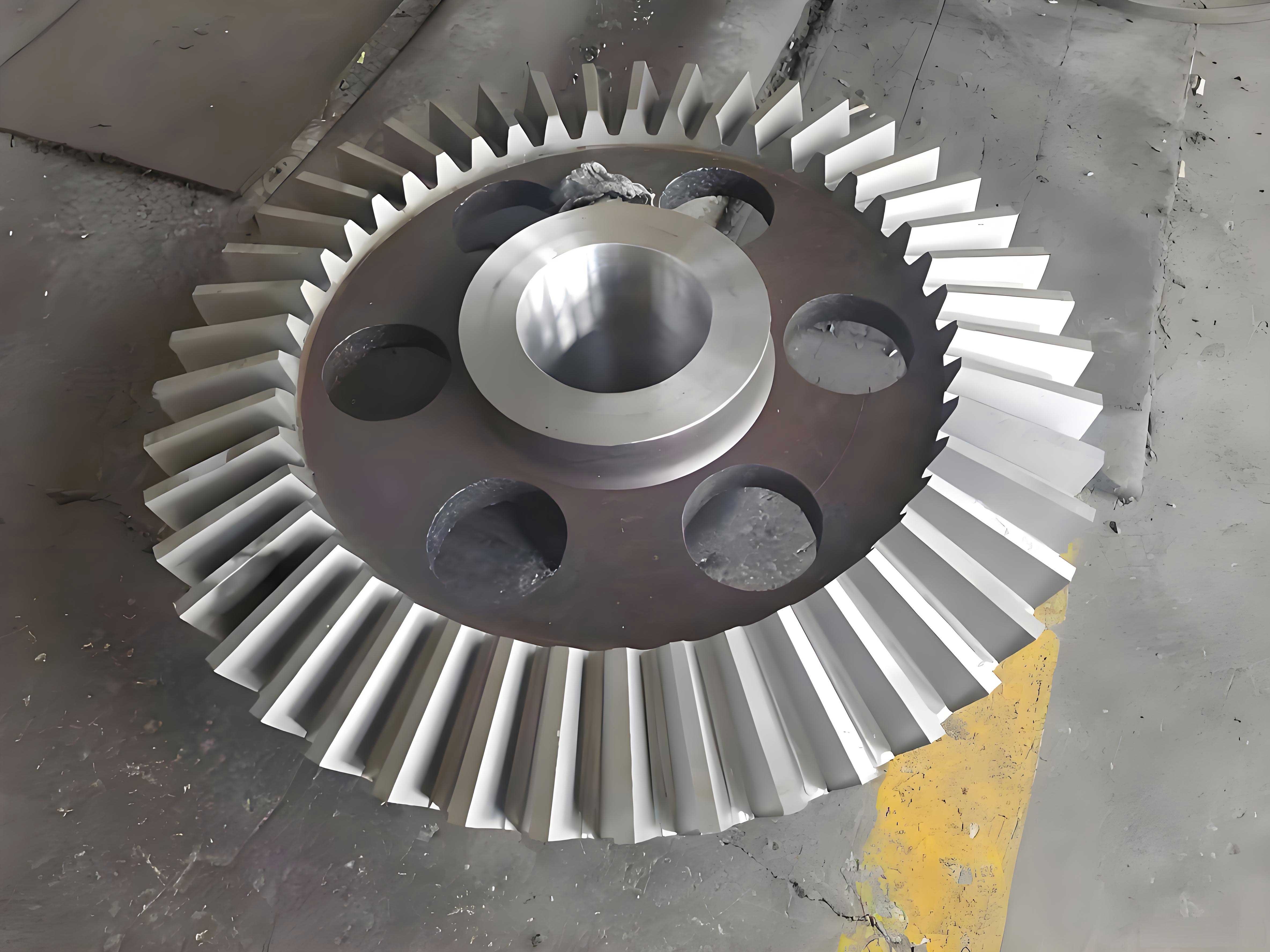
The machining of large-module straight bevel gears, often referred to as miter gears when the shaft angle is 90 degrees and the gear ratio is 1:1, presents a significant challenge in heavy machinery manufacturing. Traditional methods include form milling, template copying, and generating processes like planing or grinding. A common characteristic of these methods is their reliance on approximating the true spherical involute tooth flank with a planar involute profile developed on the gear’s back-cone. For large-module miter gears, the use of an indexable form milling cutter, often called a finger-type cutter, offers a distinct and practical alternative. This method completes a tooth space in a single pass, providing higher productivity and the flexibility to be performed on general-purpose milling machines. It is particularly economical for repair shops or situations with limited access to dedicated gear-cutting equipment. While the inherent accuracy of this method is lower compared to generating processes, large-module miter gears typically have lower precision requirements. By rationally selecting the cutter, adjusting machining parameters, and applying necessary cutter profile modifications, the resulting gears can satisfactorily meet service demands. Although this technique has been applied in practice, detailed analyses concerning cutter modification, quantitative error assessment between the machined profile and the theoretical profile are scarce. This article aims to provide a detailed computer-aided analysis and calculation methodology to enhance the practical application level of machining miter gears with indexable milling cutters.
The foundation for analyzing the machining of miter gears lies in defining the reference tooth profile. According to gear meshing theory, the exact tooth surface equation of a bevel gear can be derived. Its intersection with the back-cone surface yields the theoretical tooth profile on that cone. However, this approach is complex and offers limited practical value for this machining method. Therefore, it remains standard to use the involute on the back-cone as the correct reference profile. Consider a miter gear with standard module \( m \), large-end module \( m_e \), number of teeth \( z \), and pitch cone distance \( R \). At any axial distance \( s \) from the standard module’s back-cone surface (where positive \( s \) reduces the cone distance \( R \)), the reference profile module \( m_s \) can be derived from the constancy of the virtual number of teeth across all back-cones:
$$ m_s = m \frac{R + s}{R} $$
where the virtual number of teeth \( z_v \) is \( z / \cos \delta \), and \( \delta \) is the pitch cone angle. Consequently, the reference tooth profile on any back-cone section of the miter gear is represented by an involute defined by module \( m_s \) and the standard pressure angle \( \alpha \). If the pressure angle at the standard module section is \( \alpha \), and the involute roll angle is \( \theta = \tan \alpha – \alpha \), then for the profile on a section with module \( m_s \) to have the same roll angle \( \theta \), its pressure angle \( \alpha_s \) must also be \( \alpha \). Therefore, the reference profile pressure angle is constant across the face width of the miter gear: \( \alpha_s = \alpha \).
During the milling process, the axis of the indexable milling cutter must be perpendicular to the pitch cone line of the miter gear. Once the cutter is selected, the resulting tooth profile on different back-cone sections is determined solely by the cutter’s profile and the depth of cut (or a slight rotation of the cutter axis). This analysis focuses on variations in the depth of cut. The general principle is to ensure the actual chordal tooth space width at the pitch circle matches the reference chordal space width. This condition allows us to calculate the required variation in cutting depth, \( \Delta h \) (defined as positive when the cut becomes shallower).
Let us establish the coordinate systems, as shown in the conceptual diagram. In a given cross-section at a distance \( s \) from the standard reference plane, we select a cutter with module \( m_0 \), number of teeth \( z_0 \), and pressure angle \( \alpha_0 \). The chordal tooth thickness of this cutter at its pitch circle, \( S_{t0} \), is given by:
$$ S_{t0} = m_0 z_0 \sin(\frac{\pi – S_{a0}/r_0}{z_0}) $$
where \( S_{a0} \) is the chordal addendum thickness, \( r_0 \) is the cutter’s pitch radius, and the calculation involves the involute start angle and roll angle. On the miter gear, at the same axial location \( s \), the reference chordal tooth space width at the pitch circle is \( W_s \):
$$ W_s = m_s z_v \sin(\frac{\pi – S_{as}/r_s}{z_v}) $$
Here, \( r_s \) is the pitch radius of the reference profile in that section, \( z_v \) is the virtual number of teeth, and \( S_{as} \) is the corresponding chordal addendum. To match the space width, the effective cutter center must be offset. The resulting cutting depth change \( \Delta h \) is calculated from the difference between the reference space width and the cutter’s chordal thickness, factoring in the geometry. The relationship is not linear with \( s \). To simplify setup, a linear approximation can be used. The total depth change from the small end (\( \Delta h_{small} \)) to the large end (\( \Delta h_{large} \)) is calculated, and a linear taper is applied over the gear face width \( b \). The slope \( k \) of this depth change is:
$$ k = \frac{\Delta h_{large} – \Delta h_{small}}{b} $$
or alternatively, if the cutter’s reference section is at a distance \( p \) from the large end:
$$ k’ = \frac{\Delta h_{large}}{p} = \frac{-\Delta h_{small}}{b – p} $$
The core of the analysis is the comparison between the actual machined profile and the reference profile. We establish two coordinate systems: \( O-xy \) for the reference profile (with the y-axis along the tooth space symmetry line) and \( O_0-x_0y_0 \) for the cutter profile. For a given section, when the depth change \( \Delta h(s) \) is applied, the origins of these systems are offset by a calculated distance \( \Delta \) along the y-direction. The equation of the reference profile (right flank) in the \( O-xy \) system is:
$$ \begin{cases}
x = r_{bs}(\cos(\phi + \theta_s) + (\phi + \theta_s)\sin(\phi + \theta_s)) \\
y = r_{bs}(\sin(\phi + \theta_s) – (\phi + \theta_s)\cos(\phi + \theta_s))
\end{cases} $$
where \( r_{bs} \) is the base circle radius of the reference profile in that section, \( \phi \) is the roll parameter, and \( \theta_s \) is the starting angle. The equation of the cutter profile (which becomes the actual gear tooth flank) in the \( O-xy \) system is a transformed version of its own involute equation, incorporating the offset \( \Delta \). By solving these equations for the same x-coordinate, we can find the error in the y-direction, \( \Delta y = y_{actual} – y_{reference} \). This error serves as the primary basis for cutter profile modification.
However, the y-direction error does not directly reflect meshing performance. Transmission error is propagated along the common normal line. Therefore, calculating the error in the profile normal direction is crucial. For a point \( P(x_0, y_0) \) on the reference profile, the equation of the normal line is constructed. The intersection point of this normal line with the actual (cutter) profile is then found. The normal direction error \( \Delta_n \) is the distance between point \( P \) and this intersection point, measured along the normal line. The sign of \( \Delta_n \) indicates whether the actual profile is undercut (negative) or overshoots (positive) the reference profile.
| Error Type | Direction | Significance | Calculation Basis |
|---|---|---|---|
| Y-direction Error (\( \Delta y \)) | Along tooth space symmetry axis | Direct geometric deviation; basis for cutter regrinding. | Difference in y-coordinates for same x. |
| Normal Error (\( \Delta_n \)) | Along the tooth profile normal | True meshing error; determines transmission quality and interference. | Distance from reference point to actual profile along the normal line. |
The selection and modification of the indexable milling cutter are critical steps. The cutter’s nominal module can be chosen between the small-end and large-end modules of the miter gear, and the cutter tooth count can be varied. Different combinations yield different error patterns. Generally, selecting a cutter module close to the mean module and a tooth count close to the gear’s virtual number of teeth provides a good starting point. For narrow miter gears with low requirements, simply adjusting the depth-of-cut variation may suffice. For wider face widths, cutter profile modification becomes necessary. Modification is primarily applied to regions of the cutter profile outside the meshing zone for the selected reference section. The meshing zone itself is adjusted via depth-of-cut variation and minimal modification to avoid significant degradation of the active profile.
After modifying the cutter, its new profile, often obtained from a template, should be curve-fitted (e.g., using a least-squares cubic polynomial) to obtain an analytical expression \( y = f(x) \). This function replaces the original cutter involute equation in the error calculation procedures described above. Iterative calculations or optimization algorithms can then be used to refine the modified profile until the error criteria are met for the miter gear.
A significant advantage emerges when machining a pair of mating miter gears. Analyzing and modifying cutters for each gear independently can lead to large modifications and significant residual errors. A paired approach considers both gears simultaneously, allowing errors to compensate for each other. The method allows a controlled amount of interference (negative normal error) on each gear, provided that the sum of the normal errors of the two mating profiles at any contact point is greater than or equal to zero. This condition ensures no physical interference occurs during meshing. This paired analysis can often reduce or even eliminate the need for cutter modification. To implement this, the lines of action on both gears are determined. For any point on the line of action, the corresponding contact radii \( \rho_1 \) and \( \rho_2 \) on the two miter gears are calculated using the fundamental gear meshing equation:
$$ \rho_1 = \frac{a’ \sin \alpha’}{\sin(\alpha’ + \varphi)}, \quad \rho_2 = \frac{a’ \sin \alpha’}{\sin(\alpha’ – \varphi)} $$
where \( a’ \) is the operating center distance on the back-cone, \( \alpha’ \) is the operating pressure angle, and \( \varphi \) is an angular parameter along the line of action. The normal errors \( \Delta_{n1} \) and \( \Delta_{n2} \) at these radii are computed. The non-interference condition is \( \Delta_{n1} + \Delta_{n2} \ge 0 \). Adjustments to depth-of-cut and/or cutter profiles are made until this condition is satisfied across the entire contact path.
| Parameter | Gear 1 & 2 Value | Description |
|---|---|---|
| Number of Teeth (\( z \)) | 30 | For a 1:1 ratio miter gear pair. |
| Module (Large End) (\( m_e \)) | 20 mm | Defines the gear size. |
| Face Width (\( b \)) | 200 mm | Width of the gear tooth. |
| Pitch Cone Angle (\( \delta \)) | 45° | For a 90° shaft angle. |
| Pressure Angle (\( \alpha \)) | 20° | Standard tooth profile angle. |
| Virtual Number of Teeth (\( z_v \)) | ≈42.43 | \( z / \cos \delta \). |
| Reference Modules (\( m_s \)) | Small: 16mm, Mean: 18mm, Large: 20mm | Calculated across the face width. |
For a pair of large-module miter gears with the parameters above, a standard module indexable cutter (e.g., \( m_0 = 18 \) mm) can be selected. Without modification, and using a linear depth-of-cut variation calculated only from end conditions, interference occurs in the mesh. A simple adjustment, such as increasing the cut depth slightly at the small end to introduce pitch circle clearance, can eliminate interference, but the maximum normal error might be as high as 0.3 mm. To improve quality, individual cutter modification targeting zero interference for each miter gear can reduce the maximum normal error to below 0.1 mm. However, employing the paired analysis and modification strategy allows the sum of normal errors for the mating pair to be kept below 0.05 mm, significantly improving meshing quality with potentially less complex cutter modifications. This analytical approach has been validated in practice; a pair of miter gears machined using this methodology has been in successful operation in a rolling mill drive for nearly a year.
In conclusion, the method of machining miter gears with indexable milling cutters, supported by the comprehensive analysis presented here, offers a fast, flexible, and practical solution validated in industrial applications. Performing error calculations across the entire tooth flank is essential for understanding real performance. Intentionally allowing a small amount of pitch line clearance at the small end during depth-of-cut setup can help minimize or eliminate meshing interference. Most importantly, the inherent machining errors from this process for a pair of miter gears are complementary. Exploiting this characteristic through paired analysis is the key to minimizing cutter modification efforts and maximizing the final meshing precision of the miter gear drive.
| Processing Step | Key Action | Objective | Tool/Method |
|---|---|---|---|
| 1. Setup & Selection | Select cutter module \( m_0 \) and tooth count \( z_0 \); align cutter axis perpendicular to pitch cone. | Establish baseline geometry for machining the miter gear. | Standard cutter catalog; machine setup. |
| 2. Depth Calculation | Calculate linear depth-of-cut variation \( \Delta h(s) \) based on matching reference chordal space width. | Ensure correct tooth space width at the pitch circle across the face width. | Geometric formulas; linear approximation. |
| 3. Error Analysis | Compute y-direction error \( \Delta y \) and normal direction error \( \Delta_n \) against reference profile. | Quantify machining inaccuracies for a single miter gear. | Coordinate transformation & intersection calculations. |
| 4. Paired Gear Analysis | Calculate normal errors \( \Delta_{n1} \) and \( \Delta_{n2} \) for mating pair along line of action. | Assess meshing quality and check for interference (\( \Delta_{n1}+\Delta_{n2} < 0 \)). | Gear meshing equations; error superposition. |
| 5. Cutter Modification | Iteratively adjust cutter profile template based on error analysis (single or paired). | Minimize normal error or error sum to meet design tolerance for the miter gears. | Curve fitting; iterative/optimization algorithms. |
| 6. Validation & Machining | Re-calculate errors with modified cutter profile; proceed with production. | Confirm performance before final machining of the miter gears. | Software simulation; physical cutting test. |
The successful application of this analytical framework demonstrates that viable miter gears for heavy-duty applications can be produced efficiently using standard milling equipment. Future work could integrate this analysis into CAM software for automated toolpath generation and cutter profile optimization, further bridging the gap between theoretical gear design and practical manufacturing of miter gears.