
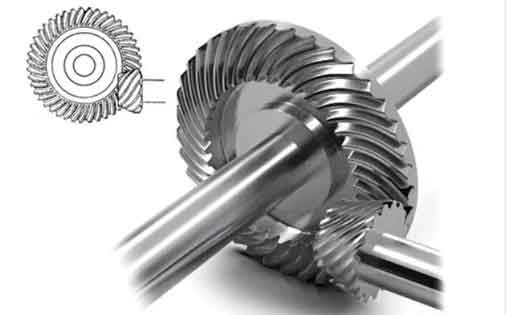
The precise and reliable operation of power transmission systems in critical applications, such as aerospace and high-performance automotive drivetrains, is paramount. Among the key components in these systems are spiral bevel gears and their close relatives, hypoid gears. Their primary advantage lies in their ability to transmit motion and power between intersecting or offset, non-parallel shafts smoothly and efficiently, thanks to their curved teeth and gradual engagement characteristics. This results in high load capacity, reduced noise, and superior performance compared to straight bevel gears. However, this performance is intrinsically linked to the perfect geometry and surface integrity of the gear teeth. Even minor deviations from the ideal tooth flank can lead to significant issues like increased vibration, noise, premature wear, and in severe cases, catastrophic failure.
One particularly insidious type of manufacturing or handling defect is a surface bump. A bump is a localized protrusion on the tooth flank, typically caused by inadvertent impact during machining, transportation, or assembly processes. Visually, these imperfections can be extremely subtle and difficult to detect with the naked eye, yet their presence disrupts the designed conjugate meshing action. Under load, as the contact ellipse expands, this bump can intrude into the nominal contact zone, causing a sudden, localized spike in contact pressure and inducing anomalous dynamic excitations. Therefore, developing a robust, systematic method for detecting the presence and location of such bumps on spiral bevel gears is a crucial step in quality assurance and performance prediction.
This article presents a detailed, first-principles methodology for detecting surface bumps on spiral bevel gears under light load conditions. The core idea is to systematically probe the entire active tooth surface by deliberately shifting the gear meshing position and analyzing the resulting transmission error (TE) signals. Transmission error, defined as the deviation of the output gear’s position from its theoretically perfect location given the input rotation, is a highly sensitive indicator of meshing quality and the presence of geometric imperfections. The method involves a synergistic combination of theoretical modeling, numerical simulation, and experimental validation. We will establish the mathematical framework for gear meshing and contact path control, detail a strategic path-planning algorithm for full-tooth-surface coverage, perform simulation via Tooth Contact Analysis (TCA), and finally, validate the approach through controlled rolling tests on a gear measurement machine.
Theoretical Foundation: Modeling Gear Meshing and Contact Control
The first step in our methodology is to establish a precise mathematical model of the spiral bevel gear pair. This model must encapsulate the geometry of the tooth flanks and the kinematic relationship between the gears under varying assembly conditions.
Mathematical Representation of Tooth Flanks
The complex geometry of a spiral bevel gear tooth is generated through a sophisticated machining process, typically using a cradle-style hypoid generator or a modern CNC machine. The surface can be described mathematically by starting with the cutting tool surface and applying a series of coordinate transformations that mirror the machine kinematics. The final tooth surface for both the pinion (gear 1) and the gear (gear 2) is represented as a vector function of two parameters, often related to the cutter rotation and the generating roll angle.
Let us denote the position vector of a point on the pinion tooth surface as $ \mathbf{r}_1(\theta_1^*, \phi_p^*) $ and on the gear tooth surface as $ \mathbf{r}_2(\theta_2^*, \phi_g^*) $. Their corresponding unit normal vectors are $ \mathbf{n}_1(\theta_1^*, \phi_p^*) $ and $ \mathbf{n}_2(\theta_2^*, \phi_g^*) $. The parameters $ \theta_i^* $ and $ \phi_i^* $ are the generating motion parameters specific to the manufacturing setup.
To analyze meshing, these surfaces must be brought into a common reference frame. We define a fixed coordinate system $ S_h $ and coordinate systems $ S_1 $ and $ S_2 $ rigidly attached to the pinion and gear, respectively. The assembly configuration is defined by three critical installation parameters:
1. Offset (V): The perpendicular distance between the gear and pinion axes (crucial for hypoid gears, zero for pure spiral bevel gears).
2. Pinion Setting (H): The axial installation distance of the pinion.
3. Gear Setting (J): The axial installation distance of the gear.
The transformation from the pinion coordinate system $ S_1 $ to the fixed system $ S_h $ involves a rotation by the pinion’s mesh rotation angle $ \varphi_1 $ and a translation by $ H $. Similarly, transforming from the gear system $ S_2 $ to $ S_h $ involves a rotation by the gear’s mesh angle $ \varphi_2 $, a translation by $ J $ and $ V $, and a rotation by the shaft angle $ \Sigma $. The transformation matrices $ \mathbf{M}_{h1} $, $ \mathbf{M}_{hd} $, and $ \mathbf{M}_{d2} $ encapsulate these operations.
$$ \mathbf{M}_{h1} = \begin{bmatrix}
1 & 0 & 0 & H \\
0 & \cos\varphi_1 & \sin\varphi_1 & 0 \\
0 & -\sin\varphi_1 & \cos\varphi_1 & 0 \\
0 & 0 & 0 & 1
\end{bmatrix} $$
$$ \mathbf{M}_{hd} = \begin{bmatrix}
\cos\Sigma & 0 & \sin\Sigma & 0 \\
0 & 1 & 0 & 0 \\
-\sin\Sigma & 0 & \cos\Sigma & 0 \\
0 & 0 & 0 & 1
\end{bmatrix} $$
$$ \mathbf{M}_{d2} = \begin{bmatrix}
\cos\varphi_2 & 0 & -\sin\varphi_2 & -J \\
0 & 1 & 0 & V \\
\sin\varphi_2 & 0 & \cos\varphi_2 & 0 \\
0 & 0 & 0 & 1
\end{bmatrix} $$
Thus, the pinion and gear surfaces expressed in the common frame $ S_h $ are:
$$ \mathbf{r}_h^{(1)}(\theta_1^*, \phi_p^*, \varphi_1, H) = \mathbf{M}_{h1} \mathbf{r}_1(\theta_1^*, \phi_p^*) $$
$$ \mathbf{r}_h^{(2)}(\theta_2^*, \phi_g^*, \varphi_2, J, V) = \mathbf{M}_{hd} \mathbf{M}_{d2} \mathbf{r}_2(\theta_2^*, \phi_g^*) $$
Their unit normals are transformed using the $3 \times 3$ linear rotation sub-matrices $ \mathbf{L} $ of the corresponding transformation matrices.
Conditions of Conjugate Meshing and Contact Path Control
For a point on the pinion to be in perfect contact with a point on the gear at a given instant, two fundamental conditions must be satisfied simultaneously:
1. Position Continuity: The position vectors of the contacting points must be equal.
2. Normal Vector Continuity: The unit normal vectors at the contacting points must be collinear (opposite in direction for driving and driven surfaces).
This yields the system of vector equations:
$$ \mathbf{r}_h^{(1)}(\theta_1^*, \phi_p^*, \varphi_1, H) = \mathbf{r}_h^{(2)}(\theta_2^*, \phi_g^*, \varphi_2, J, V) $$
$$ \mathbf{n}_h^{(1)}(\theta_1^*, \phi_p^*, \varphi_1) = -\mathbf{n}_h^{(2)}(\theta_2^*, \phi_g^*, \varphi_2) $$
Additionally, the meshing law, derived from the requirement that the relative velocity at the contact point has no component along the common normal, provides the scalar equation of meshing:
$$ \mathbf{n}_h^{(2)} \cdot \mathbf{v}_h^{(12)} = f(\theta_1^*, \phi_p^*, \varphi_1, \theta_2^*, \phi_g^*, \varphi_2, V, H, J) = 0 $$
where $ \mathbf{v}_h^{(12)} $ is the relative velocity vector.
Finally, the axial adjustments $ H $, $ J $, and $ V $ are not independent if a specific working backlash or mounting distance is to be maintained. An approximate relational constraint, derived from the spatial geometry of the gear set, can be expressed as:
$$ H + J \tan \delta_2 + \sqrt{r_2^2 + E^2} – \sqrt{r_2^2 – V^2} = 0 $$
where $ \delta_2 $ is the gear pitch cone angle, $ r_2 $ is the gear pitch radius, and $ E $ is the nominal offset.
The system of equations above has seven unknowns ($ \theta_1^*, \phi_p^*, \varphi_1, \theta_2^*, \phi_g^*, \varphi_2 $ and one of $ V, H, J $ linked by the constraint) and seven equations (three from position equality, two from independent normal equality, one meshing equation, one constraint). This system can be solved numerically, for instance using iterative methods in MATLAB. The solution provides the functional relationship $ \varphi_2(\varphi_1) $ for a given set of $ (V, H, J) $.
The Central Principle for Bump Detection: By intentionally varying the assembly parameters $ V $, $ H $, and $ J $ from their nominal values, we can deliberately shift the path of contact, i.e., the zone where the teeth theoretically make contact, across the tooth flank of the spiral bevel gear. If we have a predetermined target contact point location on the gear tooth (defined by its longitudinal and profile coordinates $ s_1 $ and $ s_2 $), we can solve the inverse problem: calculate the specific $ V $, $ H $, $ J $ adjustments required to bring the contact ellipse center to that target point under light load. This forms the basis for our probing strategy.
Strategic Path Planning for Full-Surface Interrogation
A random or ad-hoc adjustment of contact position is inefficient and may leave areas of the tooth flank untested. Therefore, a systematic path-planning strategy is essential to ensure comprehensive coverage of the entire active tooth surface of the spiral bevel gear. The goal is to define a series of target contact center points such that, by sequentially adjusting the meshing parameters to these targets, we effectively “scan” the tooth for anomalies.
The planning must consider practical constraints:
1. The contact ellipse should not run off the edges of the tooth to avoid edge contact and false readings.
2. The path should cover areas most likely to be involved in loaded contact.
3. The number of probe positions should be optimized for efficiency while maintaining adequate resolution.
A robust strategy involves dividing the tooth flank into a grid of probe zones. A practical implementation for a spiral bevel gear tooth is illustrated conceptually below. The active surface is bounded by the tip, root, toe (inner end), and heel (outer end) lines. A margin, typically 5% of the face width and tooth depth, is reserved from these edges to define the safe probing boundary.
We propose a path consisting of seven critical probe positions, which can be visualized as moving the contact center along two distinct traverses starting from a central-midface location (Position 1).
Traverse A (Towards Toe): From Position 1 (mid-face), move the contact towards the tip (Position 2), then to the toe-tip corner (Position 3), and finally down to the toe-root corner (Position 4).
Traverse B (Towards Heel): Reset to nominal and start again from Position 1. Move the contact towards the root (Position 5), then to the heel-root corner (Position 6), and finally up to the heel-tip corner (Position 7).
This 7-point path, as summarized in the table below, ensures that the central regions as well as all four critical corners of the spiral bevel gear tooth are probed, providing a high degree of confidence in full-surface coverage.
| Position ID | Description on Gear Tooth Flank | Primary Adjustment Goal |
|---|---|---|
| 1 | Central, mid-face (reference point) | Establish baseline TE |
| 2 | Mid-face, towards tip | Probe upper mid-face region |
| 3 | Toe-side, near tip | Probe toe-tip corner region |
| 4 | Toe-side, near root | Probe toe-root corner region |
| 5 | Mid-face, towards root | Probe lower mid-face region |
| 6 | Heel-side, near root | Probe heel-root corner region |
| 7 | Heel-side, near tip | Probe heel-tip corner region |
Numerical Simulation via Tooth Contact Analysis (TCA)
Before conducting physical experiments, it is imperative to simulate the process using Tooth Contact Analysis. TCA software, which can be implemented in environments like MATLAB, solves the system of meshing equations numerically. For our purpose, we use it in two modes:
1. Forward TCA: Given a set of assembly errors ($ \Delta V, \Delta H, \Delta J $), predict the contact pattern location and transmission error.
2. Inverse TCA (Our Use Case): Given a desired contact center location (from our path plan), calculate the required $ \Delta V, \Delta H, \Delta J $ adjustments.
Let’s consider a hypoid gear pair example (a generalized case of spiral bevel gears with an offset). The basic geometric and manufacturing parameters are summarized below. The analysis focuses on the drive side contact (e.g., pinion concave flank mating with gear convex flank).
| Parameter | Pinion | Gear |
|---|---|---|
| Number of Teeth | 8 | 39 |
| Module (mm) | 7.564 | — |
| Shaft Angle (°) | 90 | |
| Offset (mm) | 25.4 | |
| Mean Spiral Angle (°) | 45.04 | 33.55 |
| Hand of Spiral | Left | Right |
Running the inverse TCA for each of the seven target positions yields the specific machine setting adjustments required. The following table presents a simulated result of these calculations. It’s observed that the gear setting $J$ has minimal impact on contact location for small adjustments and is primarily used for backlash control, while $V$ and $H$ are the primary controls.
| Pos. ID | $\Delta V$ (mm) | $\Delta H$ (mm) | $\Delta J$ (mm) (for constant backlash) |
|---|---|---|---|
| 1 (Nominal) | 0.000 | 0.000 | 0.000 |
| 2 | +0.012 | -0.045 | -0.008 |
| 3 | -0.085 | -0.120 | +0.015 |
| 4 | -0.110 | +0.065 | +0.022 |
| 5 | -0.008 | +0.038 | -0.005 |
| 6 | +0.095 | +0.105 | -0.018 |
| 7 | +0.125 | -0.090 | -0.025 |
Furthermore, forward TCA can be run for each adjusted position to predict the nominal, or “bump-free,” transmission error. The Transmission Error for a single mesh cycle is calculated as:
$$ \Delta \varphi(\varphi_1) = \left( \varphi_2(\varphi_1) – \varphi_{20} \right) – \frac{z_1}{z_2} \left( \varphi_1 – \varphi_{10} \right) $$
where $z_1, z_2$ are tooth numbers, and $\varphi_{10}, \varphi_{20}$ are initial reference angles. The peak-to-peak amplitude of this TE curve for each probe position under ideal conditions serves as the baseline for comparison. A typical simulation result might show amplitudes ranging from a few arc-seconds in the central region to perhaps ten arc-seconds near the corners due to more severe unloaded conjugacy conditions.
| Position ID | Simulated TE Amplitude (arc-seconds) |
|---|---|
| 1 | 4.2 |
| 2 | 5.9 |
| 3 | 5.6 |
| 4 | 6.1 |
| 5 | 4.1 |
| 6 | 8.4 |
| 7 | 9.7 |
Experimental Validation through Rolling Test
The practical validation of this methodology is performed on a high-precision gear rolling and testing machine, such as a YX-HTT600 type gear integrated error tester. This machine allows for precise, CNC-controlled adjustment of the $V$, $H$, and $J$ axes while measuring the rotational angles of both the driving and driven spindles with high-resolution encoders.
Experimental Procedure
- Gear Mounting: The hypoid or spiral bevel gear pair is mounted on the test machine’s spindles.
- Path Execution: Starting from a nominal position (Pos. 1), the machine settings are adjusted according to the values derived from the inverse TCA simulation (Table 3) to sequentially achieve the seven probe positions.
- Contact Verification: At each position, a light marking compound (e.g., Prussian blue) is applied to several gear teeth. The gears are rolled under very light load to imprint the contact pattern. This visual check confirms that the contact ellipse has indeed been moved to the intended zone on the spiral bevel gear tooth flank.
- Data Acquisition: With the marking compound cleaned off, the gears are rolled again at each fixed position. The angular position signals from both encoders are sampled synchronously at a high rate.
- Signal Processing: The raw data is processed to compute the static transmission error $ \Delta \varphi(\varphi_1) $ for one complete revolution of the gear, isolating individual tooth meshing events.
Bump Detection Logic and Results Analysis
The core of the detection algorithm lies in comparing the measured TE signal at each probe position against the expected nominal TE from the simulation. Under ideal, bump-free conditions, the measured TE amplitude for a given position should closely match the simulated amplitude, albeit with some variation due to inherent manufacturing micro-errors and measurement noise.
The presence of a bump within the active contact zone of a specific probe position will cause a significant local disturbance in the TE curve. As the gears mesh and the contact traverses the bump, a sharp, anomalous spike will appear in the TE signal for that particular tooth. The key indicators are:
1. Amplitude Deviation: The peak-to-peak amplitude of the measured TE for the problematic position will significantly exceed the simulated nominal amplitude. A threshold, e.g., 20% above the nominal amplitude, can be set to flag a potential bump.
2. Localized Spike: Within the TE waveform for one revolution, a single, pronounced spike will correspond to the precise angular position (i.e., the specific tooth number) where the bump is located.
Example Experimental Result: Suppose during the rolling test, the TE curves for positions 1 through 5 show good agreement with simulation. However, at Position 6 (heel-root probe), the measured TE amplitude is found to be 29.9 arc-seconds, which is over 250% of the simulated nominal amplitude of 8.4 arc-seconds for that position. Furthermore, examining the TE waveform for the revolution at Position 6 reveals a large, isolated spike occurring at the mesh cycle corresponding to, say, tooth number 6 on the gear. This provides compelling evidence that a surface bump exists on tooth #6, specifically in the heel-root region of its flank. Similarly, a spike at Position 1 might indicate a bump in the central region of a tooth.
| Position ID | Sim. TE Amp. [“] | Meas. TE Amp. (Good Gear) [“] | Meas. TE Amp. (Faulty Gear) [“] | Detection Flag (20% Threshold) | Inferred Bump Location |
|---|---|---|---|---|---|
| 1 | 4.2 | 4.4 | 4.5 | No | — |
| 2 | 5.9 | 6.8 | 6.5 | No | — |
| 3 | 5.6 | 6.3 | 27.4 | YES | Tooth #6, Toe-Tip area |
| 4 | 6.1 | 6.7 | 6.9 | No | — |
| 5 | 4.1 | 4.2 | 4.3 | No | — |
| 6 | 8.4 | 9.7 | 29.9 | YES | Tooth #6, Heel-Root area |
| 7 | 9.7 | 10.8 | 11.1 | No | — |
The method’s resolution is limited by the size of the contact ellipse and the noise floor of the measurement system. Very subtle bumps might not produce a detectable signal exceeding the threshold, especially if they are located in regions where the nominal unloaded conjugacy is already poor (e.g., corners, leading to higher nominal TE). However, for significant bumps that would realistically affect performance under load, this method provides a clear, quantitative, and localizing detection capability.
Conclusion
This article has detailed a systematic methodology for the detection of surface bumps on spiral bevel gears. The approach integrates fundamental gear geometry, controlled meshing parameter adjustment, numerical simulation, and precision metrology. The key steps involve: establishing a mathematical model for contact path control; planning an efficient probing path to cover the entire active tooth flank; using TCA to calculate the necessary machine setting adjustments ($V, H, J$) to execute this path; and finally, conducting rolling tests to measure transmission error at each probe position.
The detection is based on the principle that a localized surface imperfection will cause a significant, identifiable anomaly in the transmission error signal when the contact zone is positioned over it. By systematically moving the contact zone according to the planned path, every region of the spiral bevel gear tooth can be interrogated. The correlation between a specific probe position and a spike in the TE curve allows for not only detecting the presence of a bump but also pinpointing its approximate location on the tooth flank and identifying the affected tooth number.
This methodology provides a powerful tool for quality control and failure analysis of high-precision spiral bevel gears. It moves beyond subjective visual inspection to an objective, data-driven assessment of surface integrity. Future work could focus on automating the entire process, from path planning and TCA calculation to machine control and TE signal classification using machine learning algorithms, further enhancing the efficiency and reliability of spiral bevel gear inspection.