
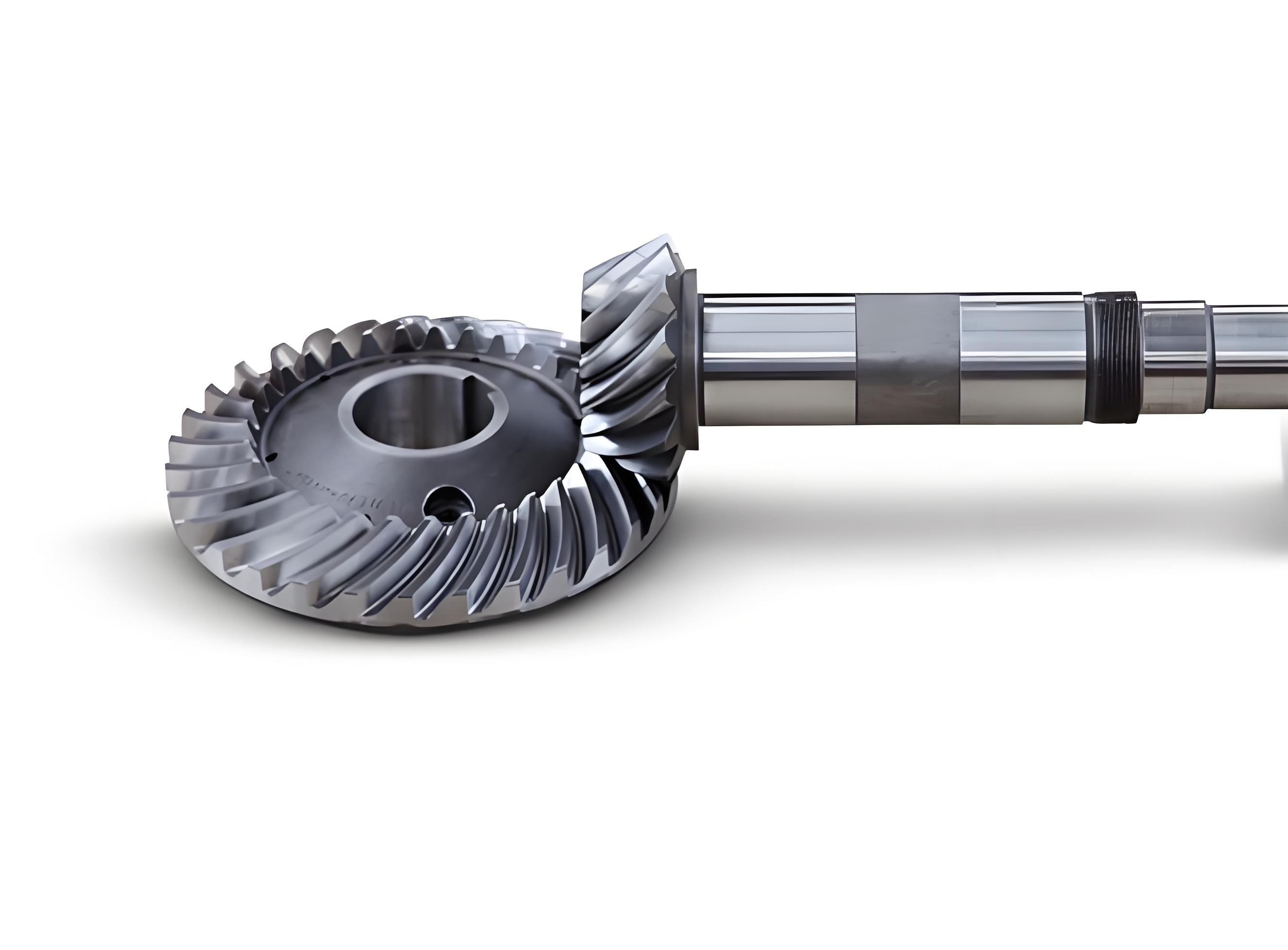
In the field of mechanical power transmission, spiral bevel gears play a crucial role due to their ability to transmit motion between intersecting shafts with high efficiency and load capacity. The bending stress at the tooth root is one of the most critical factors determining the fatigue life and reliability of spiral bevel gears. Accurate prediction of this stress under realistic operating conditions, including manufacturing errors, assembly misalignments, and deformations, is essential for optimal design. Traditional empirical methods, such as those developed by Gleason, rely on material mechanics and statistical corrections, but they often fail to capture the complex stress distributions influenced by actual gear geometry and loading scenarios. This limitation necessitates advanced computational techniques that balance precision and efficiency.
This article presents a novel methodology for calculating the bending stress history in spiral bevel gears using a stress influence matrix approach. By leveraging the principles of stress superposition and Saint-Venant’s principle, the method requires only a single finite element analysis (FEA) to derive the stress influence matrix, which is then combined with load distribution data from loaded tooth contact analysis (LTCA) to predict bending stresses throughout the entire meshing cycle. This approach significantly reduces computational effort while maintaining the accuracy inherent in finite element methods, making it suitable for engineering applications. The focus is on spiral bevel gears, and the term “spiral bevel gears” will be emphasized throughout to highlight its relevance.
The core of this methodology lies in the concept of a stress influence matrix. We begin by generating a finite element mesh of the spiral bevel gear tooth, including the root transition surface, based on numerical simulation of the tooth geometry using known design and manufacturing parameters. The mesh typically employs 20-node isoparametric elements for high accuracy. The stress influence matrix is defined as follows: consider a gear tooth with \(n\) nodes on the working tooth surface and \(m\) nodes on the root transition surface. When a unit normal load is applied sequentially at each of the \(n\) surface nodes, the resulting stress states at each of the \(m\) root nodes are computed. This forms a matrix \([S]_{n \times m}\), where each element \(\{\sigma\}_{ij}\) represents the stress vector at root node \(j\) due to a unit load at surface node \(i\). Mathematically, this can be expressed as:
$$[S]_{n \times m} = \begin{bmatrix} \{\sigma\}_{11} & \{\sigma\}_{12} & \cdots & \{\sigma\}_{1m} \\ \{\sigma\}_{21} & \{\sigma\}_{22} & \cdots & \{\sigma\}_{2m} \\ \vdots & \vdots & \ddots & \vdots \\ \{\sigma\}_{n1} & \{\sigma\}_{n2} & \cdots & \{\sigma\}_{nm} \end{bmatrix}$$
This matrix encapsulates the linear elastic response of the spiral bevel gear tooth and is computed once via FEA, stored as a fundamental mechanical property for subsequent stress analysis without further finite element computations.
To enhance computational efficiency and accuracy, stress reduction integration and smoothing techniques are applied. For 20-node hexahedral elements, a 2×2×2 Gaussian integration scheme is used instead of the standard 3×3×3, as it improves element behavior and reduces computation time. Stresses are first calculated at Gauss points, where precision is highest, and then smoothed to the corner nodes of each element using a least-squares approach. The transformation from Gauss point stresses \(\sigma_1, \sigma_2, \ldots, \sigma_8\) to corner node stresses \(\tilde{\sigma}_1, \tilde{\sigma}_2, \ldots, \tilde{\sigma}_8\) is given by:
$$\begin{bmatrix} \tilde{\sigma}_1 \\ \tilde{\sigma}_2 \\ \tilde{\sigma}_3 \\ \tilde{\sigma}_4 \\ \tilde{\sigma}_5 \\ \tilde{\sigma}_6 \\ \tilde{\sigma}_7 \\ \tilde{\sigma}_8 \end{bmatrix} = \begin{bmatrix} a & b & b & c & d & c & c & b \\ b & a & c & b & c & b & d & c \\ c & b & d & c & b & a & c & b \\ d & c & c & b & c & b & b & a \\ b & c & a & b & c & d & b & c \\ a & b & b & c & b & c & c & d \\ b & c & c & d & a & b & b & c \\ c & d & b & c & b & c & a & b \end{bmatrix} \begin{bmatrix} \sigma_1 \\ \sigma_2 \\ \sigma_3 \\ \sigma_4 \\ \sigma_5 \\ \sigma_6 \\ \sigma_7 \\ \sigma_8 \end{bmatrix}$$
where \(a = \frac{1}{4}(5 + 3\sqrt{3})\), \(b = -\frac{1}{4}(\sqrt{3} + 1)\), \(c = -\frac{1}{4}(\sqrt{3} – 1)\), and \(d = \frac{1}{4}(5 – 3\sqrt{3})\). Stress continuity at shared nodes is ensured by averaging stresses from adjacent elements, which mitigates discontinuities common in isoparametric formulations.
The next step involves determining the stress influence matrix for points along the contact path on the tooth surface. Using LTCA for spiral bevel gears, the contact ellipses and their pressure distributions are obtained at discrete meshing positions. The contact path is discretized into \(l\) positions, each with a contact ellipse whose major axis is sampled at \(k\) points. The stress influence matrix for these discrete points, denoted as \([\tilde{S}]_{k \times m}\), is derived from the nodal matrix \([S]_{n \times m}\) via bivariate interpolation. A coordinate system is established on the rotational projection plane (through the gear axis), with the origin at the pitch cone apex, X-axis along the pitch cone line, and Y-axis perpendicular to it. For an interpolation point \((x, y)\), the function value \(z(x, y)\) (representing stress influence) is computed using Lagrangian interpolation over nine nearby grid nodes:
$$z(x, y) = \sum_{i=p}^{p+2} \sum_{j=q}^{q+2} \left( \prod_{\substack{k=p \\ k \neq i}}^{p+2} \frac{x – x_k}{x_i – x_k} \right) \left( \prod_{\substack{l=q \\ l \neq j}}^{q+2} \frac{y – y_l}{y_j – y_l} \right) z_{ij}$$
Here, \(z_{ij} = z(x_i, y_j)\) are the stress influence values at grid nodes. This interpolation yields \([\tilde{S}]_{k \times m}\), where each element \(\{\tilde{\sigma}\}_{ij}\) is the stress at root node \(j\) due to a unit load at contact point \(i\) on the surface of the spiral bevel gear.
The bending stress history is then computed by combining the load distribution matrix with the interpolated stress influence matrix. Based on Saint-Venant’s principle, the distributed load on each contact ellipse can be replaced by an equivalent set of concentrated forces at the discrete points along the major axis. The load distribution matrix \([L]_{l \times k}\) is constructed as a block diagonal matrix, where each block \(\{\mathbf{L}_j\}^T_{k_j} = (p_1, p_2, \ldots, p_{k_j})\) represents the load magnitudes at the \(k_j\) discrete points of the \(j\)-th contact ellipse, with \(\sum_{j=1}^l k_j = k\). The stress superposition principle allows the bending stress process matrix \([\sigma]_{l \times m}\) to be calculated as:
$$[\sigma]_{l \times m} = [L]_{l \times k} [\tilde{S}]_{k \times m}$$
Each element \(\{\sigma_{ij}\}\) in this matrix denotes the stress vector at root node \(j\) when the load is applied at the \(i\)-th contact position. This matrix comprehensively captures the temporal and spatial variation of bending stresses on the root transition surface throughout the meshing cycle for spiral bevel gears.
For failure analysis, principal stresses and criterion stresses are derived from the stress vectors. The stress vector at any point is \(\{\sigma_{ij}\} = [\sigma_x, \sigma_y, \sigma_z, \tau_{yz}, \tau_{zx}, \tau_{xy}, \sigma_1, \sigma_2, \sigma_3, \sigma_c]\), where \(\sigma_1, \sigma_2, \sigma_3\) are the principal stresses computed from the stress invariants \(I_1, I_2, I_3\):
$$\begin{aligned}
I_1 &= \sigma_x + \sigma_y + \sigma_z \\
I_2 &= \sigma_x \sigma_y + \sigma_y \sigma_z + \sigma_z \sigma_x – \tau_{xy}^2 – \tau_{yz}^2 – \tau_{zx}^2 \\
I_3 &= \sigma_x \sigma_y \sigma_z + 2\tau_{xy} \tau_{yz} \tau_{zx} – \sigma_x \tau_{yz}^2 – \sigma_y \tau_{zx}^2 – \sigma_z \tau_{xy}^2
\end{aligned}$$
The principal stresses are given by:
$$\begin{aligned}
\sigma_1 &= \frac{I_1}{3} – R \cos\left(\frac{\phi}{3}\right) \\
\sigma_2 &= \frac{I_1}{3} + R \cos\left(\frac{2\pi + \phi}{3}\right) \\
\sigma_3 &= \frac{I_1}{3} + R \cos\left(\frac{4\pi + \phi}{3}\right)
\end{aligned}$$
where \(R = \frac{2}{3} \sqrt{I_1^2 – 3I_2}\) and \(\cos \phi = \frac{2I_1^3 – 9I_1 I_2 + 27I_3}{2(I_1^2 – 3I_2)^{3/2}}\). The von Mises equivalent stress \(\sigma_c\), commonly used as a yield criterion, is calculated as:
$$\sigma_c = \sqrt{\frac{(\sigma_1 – \sigma_2)^2 + (\sigma_2 – \sigma_3)^2 + (\sigma_3 – \sigma_1)^2}{2}}$$
This criterion stress is particularly useful for assessing the fatigue strength of spiral bevel gears under cyclic loading.
To demonstrate the applicability of this method, a case study involving a pair of spiral bevel gears is presented. The geometric and manufacturing parameters are summarized in the tables below, which are essential for generating the tooth surface and finite element mesh. The pinion is subjected to a torque of 1260 Nm, and LTCA is performed to obtain the load distribution.
| Parameter | Pinion | Gear |
|---|---|---|
| Number of teeth, \(z\) | 21 | 28 |
| Module, \(m\) (mm) | 10.714 | |
| Normal pressure angle, \(\alpha_n\) (°) | 20 | |
| Midpoint spiral angle, \(\beta_m\) (°) | 35 | |
| Spiral direction | Left | Right |
| Shaft angle, \(\Sigma\) (°) | 90 | |
| Pitch cone angle, \(\delta\) (°) | 36.8667 | 53.1333 |
| Face width, \(B\) (mm) | 35 | |
| Outer cone distance, \(R\) (mm) | 187.5 | |
Additional manufacturing parameters for the pinion and gear are provided in the following tables, which influence the tooth geometry and contact patterns in spiral bevel gears.
| Parameter | Concave Side | Convex Side |
|---|---|---|
| Tool tip radius, \(r_{p1}\) (mm) | 105.0624 | 123.2452 |
| Tool pressure angle, \(\alpha_1\) (°) | 18.75 | 21.25 |
| Radial setting, \(S_{r1}\) (mm) | 129.8731 | 137.516 |
| Angular setting, \(q_1\) (°) | 42.506 | 44.5606 |
| Machine roll ratio, \(m_{p1}\) | 0.6137 | 0.5897 |
| Parameter | Convex Side | Concave Side |
|---|---|---|
| Cutter diameter, \(D_{C2}\) (mm) | 228.6 | |
| Tool edge width, \(p_{w2}\) (mm) | 5.8 | |
| Tool pressure angle, \(\alpha_2\) (°) | 20 | |
| Radial setting, \(S_{r2}\) (mm) | 133.785 | |
Using the stress influence matrix method, the bending stresses are computed over the meshing cycle. The maximum tensile stress on the pinion root is found to be 54.129 MPa, and the maximum compressive stress is 75.229 MPa. For the gear, the maximum tensile stress is 86.354 MPa, and the maximum compressive stress is 114.259 MPa. The stress distribution on the root transition surface can be visualized via contour plots, illustrating the critical regions prone to fatigue failure. Additionally, the time history of tensile stress at the midpoint of the pinion tooth root is plotted against the contact position index, showing periodic fluctuations corresponding to the meshing sequence of spiral bevel gears.
The advantages of this methodology are manifold. By decoupling the finite element analysis from the load-dependent stress calculation, the computational burden is drastically reduced. The stress influence matrix, once computed, serves as a reusable database for various loading scenarios, facilitating parametric studies and optimization of spiral bevel gear designs. Moreover, the integration of LTCA ensures that realistic contact conditions, including misalignments and deformations, are accounted for, leading to more accurate stress predictions than traditional empirical formulas. This approach is particularly beneficial for high-performance applications where weight reduction and reliability are paramount, such as in aerospace and automotive transmissions involving spiral bevel gears.
In conclusion, the stress influence matrix method provides an efficient and precise framework for calculating bending stress histories in spiral bevel gears. It harnesses the power of finite element analysis while minimizing computational costs through superposition principles and interpolation techniques. The method’s ability to capture the full meshing cycle stress distribution with a single FEA makes it a practical tool for engineers designing spiral bevel gears. Future work could extend this approach to include dynamic effects, thermal loads, and material nonlinearities, further enhancing its applicability to advanced gear systems. Ultimately, the continued refinement of such computational methods will drive innovation in the design and analysis of spiral bevel gears, ensuring their optimal performance in demanding mechanical applications.
The mathematical foundations and algorithmic steps described herein underscore the importance of numerical methods in modern gear engineering. By leveraging matrices, interpolation, and superposition, we can transform complex physical problems into tractable computational tasks. This paradigm not only applies to spiral bevel gears but also to other gear types, highlighting the versatility of the stress influence matrix concept. As computational resources grow, integrating these methods with real-time simulation and digital twin technologies will pave the way for smarter, more resilient mechanical designs centered on spiral bevel gears.