
In the realm of high-power transmission systems, the precise modeling of spiral bevel gears is paramount for advanced design, dynamic simulation, and contact analysis. My focus here is to detail a methodology for constructing an exact 3D digital model of a spiral bevel gear, specifically the large wheel (gear), by rigorously emulating the kinematics of a modern NC (Numerical Control) gear-cutting machine. This approach moves beyond simplistic approximations to capture the true geometry generated by the complex relative motion between the cutting tool and the gear blank.
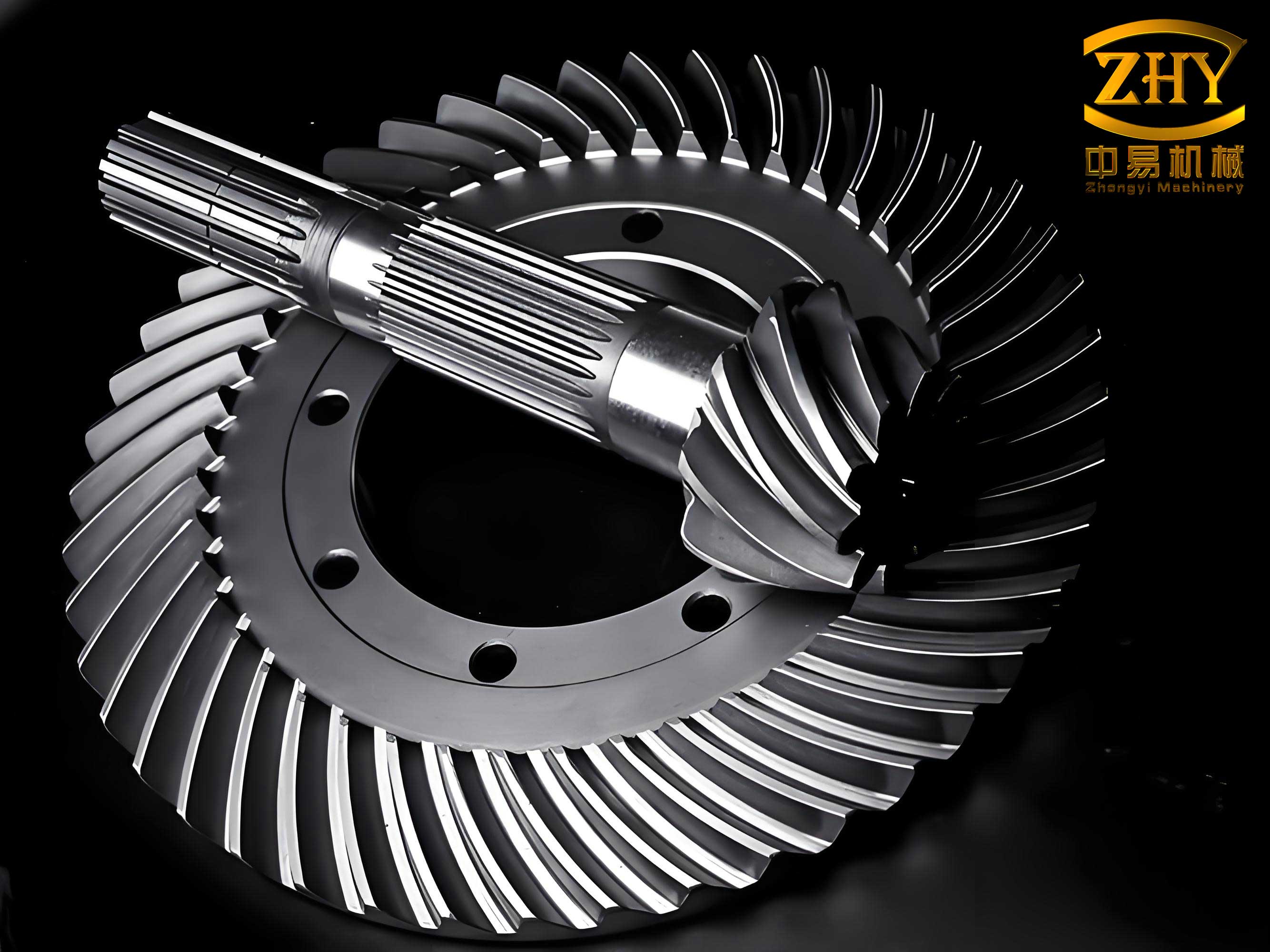
The geometry of a spiral bevel gear tooth is not a simple, predefined surface but a complex envelope generated by the motion of a cutting tool. To mathematically describe this surface, one must first establish a series of coordinate systems that represent all critical components of the machine tool and their interrelationships. These coordinate systems allow us to track the position and orientation of the cutter surface as it moves relative to the stationary gear blank. The entire machining process is conceptualized around a “phantom” generating gear, a theoretical crown gear that meshes with the workpiece. The cutting tool, mounted on a rotating cradle, represents a segment of this phantom gear’s tooth.
The following table outlines the primary coordinate systems required to model the machining process for the large spiral bevel gear.
| Coordinate System Symbol | Description | Attachment & Motion |
|---|---|---|
| $$S_{o2} = [O_{o2}; X_{o2}, Y_{o2}, Z_{o2}]$$ | Machine Frame | Fixed to the machine base. $$Z_{o2}$$ is the cradle axis. |
| $$S_{y2} = [O_{y2}; X_{y2}, Y_{y2}, Z_{y2}]$$ | Cradle Frame | Fixed to the cradle, rotates with it about $$Z_{o2}$$ by angle $$\phi_{y2}$$. |
| $$S_{d2} = [O_{d2}; X_{d2}, Y_{d2}, Z_{d2}]$$ | Cutter Head Frame | Fixed to the cutter head (not individual blades). Its orientation is set by the machine settings. |
| $$S_{f2} = [O_{f2}; X_{f2}, Y_{f2}, Z_{f2}]$$ | Auxiliary Frame 1 | Fixed, with axes parallel to $$S_{o2}$$. Facilitates transformations. |
| $$S_{a2} = [O_{a2}; X_{a2}, Y_{a2}, Z_{a2}]$$ | Auxiliary Frame 2 | Fixed to the gear blank’s theoretical initial position. $$X_{a2}$$ aligns with the gear axis. |
| $$S_{g2} = [O_{g2}; X_{g2}, Y_{g2}, Z_{g2}]$$ | Gear (Workpiece) Frame | Fixed to the gear blank, rotates with it about its own axis by angle $$\phi_{g2}$$. |
The fundamental surface generating the gear tooth is the cutting edge of the blade on the cutter head. For spiral bevel gears, a circular cutting edge is typically used, forming a conical surface. This surface, in its local cutter coordinate system $$S_{d2}$$, can be parameterized using two coordinates: the radial distance $$u_2$$ and the rotational angle $$\theta_2$$. The equation of a point on this cutting cone and its corresponding unit normal vector are given by:
$$
\mathbf{r}_{d2}(u_2, \theta_2) =
\begin{bmatrix}
(r_G – u_2 \sin \alpha_2) \cos \theta_2 \\
(r_G – u_2 \sin \alpha_2) \sin \theta_2 \\
-u_2 \cos \alpha_2
\end{bmatrix}, \quad
\mathbf{n}_{d2}(\theta_2) =
\begin{bmatrix}
\cos \alpha_2 \cos \theta_2 \\
\cos \alpha_2 \sin \theta_2 \\
-\sin \alpha_2
\end{bmatrix}
$$
Here, $$\alpha_2$$ is the cutter blade pressure angle (positive for one face, negative for the other), and $$r_G$$ is the nominal cutter point radius. In the single-indexing (Formate) process for the large spiral bevel gear, the convex and concave flanks are cut simultaneously using inner and outer blades, respectively, which is accounted for in the sign of the blade offset $$W_2/2$$: $$r_G = r_0 \pm W_2/2$$.
The heart of the modeling process lies in transforming this simple cutter surface into the complex gear tooth surface. This is achieved through a sequence of homogeneous coordinate transformations that map a point from the cutter system $$S_{d2}$$ to the gear system $$S_{g2}$$. Each transformation matrix accounts for a specific machine setting or motion.
$$
\mathbf{r}_{g2}(u_2, \theta_2, \phi_{y2}) = \mathbf{M}_{g2,a2}(\phi_{g2}) \cdot \mathbf{M}_{a2,f2} \cdot \mathbf{M}_{f2,o2} \cdot \mathbf{M}_{o2,y2}(\phi_{y2}) \cdot \mathbf{M}_{y2,d2} \cdot \mathbf{r}_{d2}(u_2, \theta_2)
$$
The matrices incorporate key machine settings such as the machine root angle $$\gamma_{m2}$$, sliding base setting $$X_{B2}$$, workpiece offset $$E_2$$, and the crucial rolling ratio $$R_{R2}$$ which links cradle rotation $$\phi_{y2}$$ to gear rotation $$\phi_{g2}$$ ($$\phi_{g2} = R_{R2} \cdot \phi_{y2}$$). The transformation chain is critical for accurately modeling spiral bevel gears.
However, the equation above describes the locus of the cutter surface in gear space, not the final envelope (the gear tooth surface). To find the envelope, we must invoke the gear meshing theory, which states that at the point of contact between the generating surface (cutter) and the generated surface (gear), their relative velocity must be perpendicular to the common surface normal. This condition is encapsulated in the meshing equation:
$$
\mathbf{n}^{(y2)} \cdot \mathbf{v}^{(y2g2)} = 0
$$
In this equation, $$\mathbf{n}^{(y2)}$$ is the surface normal vector expressed in the cradle system, and $$\mathbf{v}^{(y2g2)}$$ is the relative velocity vector between the cutter (on the cradle) and the gear workpiece, also expressed in the cradle system. Calculating this relative velocity requires considering the rotation of the cradle ($$\omega^{(y2)}$$) and the rotation of the gear ($$\omega^{(g2)}$$). Expanding this equation using the specific transformation chain eliminates the explicit velocity terms and yields a functional relationship between the surface parameters and the machine motion parameter:
$$
f(u_2, \theta_2, \phi_{y2}) = 0
$$
This meshing equation can be solved to express the radial parameter $$u_2$$ as a function of the angular parameter $$\theta_2$$ and the cradle angle $$\phi_{y2}$$: $$u_2 = u_2(\theta_2, \phi_{y2})$$. Substituting this solution back into the transformed surface equation $$\mathbf{r}_{g2}(u_2, \theta_2, \phi_{y2})$$ eliminates $$u_2$$, giving us the final mathematical definition of the spiral bevel gear tooth surface as a two-parameter family:
$$
\mathbf{r}_{g2}(\theta_2, \phi_{y2}) = [x_g(\theta_2, \phi_{y2}), \; y_g(\theta_2, \phi_{y2}), \; z_g(\theta_2, \phi_{y2})]^T
$$
With the tooth surface equation established, the next step is to compute a discrete set of points that lie on it. One cannot arbitrarily choose values for $$\theta_2$$ and $$\phi_{y2}$$; they must correspond to points that actually reside on the physically valid portion of the gear tooth, bounded by the tip, root, heel, and toe. A practical method is to project the tooth surface onto the gear’s axial plane (the $$X_{g2}O_{g2}Y_{g2}$$ plane) by defining a projected radial coordinate $$\rho = \sqrt{y_g^2 + z_g^2}$$. The valid domain in this plane is a trapezoid defined by the gear’s blank dimensions: the inner radius (heel), outer radius (toe), face apex distance, and root angle. For a given target point $$(x_{target}, \rho_{target})$$ within this domain, one solves a system of two nonlinear equations derived from the surface definition and the projection to find the corresponding $$\theta_2$$ and $$\phi_{y2}$$. This process is repeated to generate a dense point cloud.
| Gear Blank Parameter | Symbol | Example Value |
|---|---|---|
| Number of Teeth | $$N_2$$ | 42 |
| Module (at mid-face) | $$m_m$$ | 3.5 mm |
| Mean Spiral Angle | $$\beta_m$$ | 12° |
| Face Width | $$F$$ | 30 mm |
| Face Apex Distance | $$A_0$$ | 40.21 mm |
| Pitch Diameter | $$d_2$$ | 147 mm |
| Pitch Angle | $$\delta_2$$ | 60.26° |
| Machine Setting Parameter | Symbol | Example Value |
|---|---|---|
| Cutter Radius | $$r_0$$ | 44.45 mm |
| Point Width | $$W_2$$ | 2.25 mm |
| Cutter Blade Angle (Convex/Concave) | $$\alpha_2$$ | 21.25° / -18.75° |
| Machine Root Angle | $$\gamma_{m2}$$ | 57.20° |
| Sliding Base | $$X_{B2}$$ | 0 mm |
| Workpiece Offset | $$E_2$$ | 0 mm |
| Radial Setting | $$S_{r2}$$ | 74.43 mm |
| Angular Setting | $$q_2$$ | 35.74° |
| Roll Ratio | $$R_{R2}$$ | 1.15 |
In my workflow, I employ MATLAB to perform these complex calculations. I set up functions for the surface equations and the meshing condition, and then use a numerical solver like `fsolve` to find the parameters $$\theta_2$$ and $$\phi_{y2}$$ for each desired grid point on the tooth flank. The computed 3D coordinates $$(x_g, y_g, z_g)$$ are systematically saved into a text file. This file serves as the critical bridge between mathematical computation and geometric modeling.
The final stage of creating the solid model of the spiral bevel gear takes place within a CAD environment, such as SolidWorks. The process is methodical: First, the point cloud data from the text file is imported to create a set of 3D sketch points or a curve through points, effectively tracing out distinct grid lines on the tooth surface. These curves, representing the topography of the spiral bevel gear tooth, are then used as guides in a surface lofting or boundary surface command to generate a single, continuous, smooth CAD surface for the convex and concave flanks. These surfaces are trimmed and knitted together with surfaces constructed for the fillet (modeled separately based on the cutter tip) and the top land, eventually forming a closed, watertight “body” representing one solid tooth. This tooth body is then patterned circumferentially around the gear axis using a circular array. Finally, this array of teeth is combined with a base gear blank (modeled from the blank dimensions) via a Boolean subtract operation, resulting in the complete, precise 3D solid model of the spiral bevel gear.
The advantages of this kinematics-based modeling approach for spiral bevel gears are substantial. The resulting digital model is not an approximation but a true representation of the geometry that would be produced by the actual NC machining process, including the effects of all machine settings. This accuracy is indispensable for subsequent engineering analysis. For instance, the model can be directly used in Finite Element Analysis (FEA) software like ANSYS, which interfaces seamlessly with SolidWorks. An assembly of precisely modeled spiral bevel gear pairs ensures correct initial contact conditions for static stress, dynamic response, or contact fatigue studies. Furthermore, this mathematical foundation allows for the intentional modification of machine settings (e.g., slightly altering the roll ratio or cutter tilt) to perform flank corrections (ease-off), optimizing the contact pattern and transmission error under load—a critical aspect of high-performance spiral bevel gear design. In conclusion, mastering this detailed modeling process is essential for anyone involved in the advanced design, analysis, and manufacturing of high-precision spiral bevel gears.