
The pursuit of efficiency, compactness, and reliability in mechanical power transmission is a fundamental challenge in engineering design. Among various gear types, the bevel gear plays a pivotal role in applications requiring the transmission of motion and power between intersecting shafts, typically at a 90-degree angle. Their unique geometry, however, introduces specific design complexities concerning load distribution, stress concentration, and physical size. This article explores a systematic approach to the optimal design of a straight bevel gear pair, focusing on minimizing the overall volume as a primary objective to achieve a more compact and material-efficient drive system. We will establish a rigorous mathematical model, implement a solution using computational tools, and analyze the significant benefits conferred by this optimization methodology.
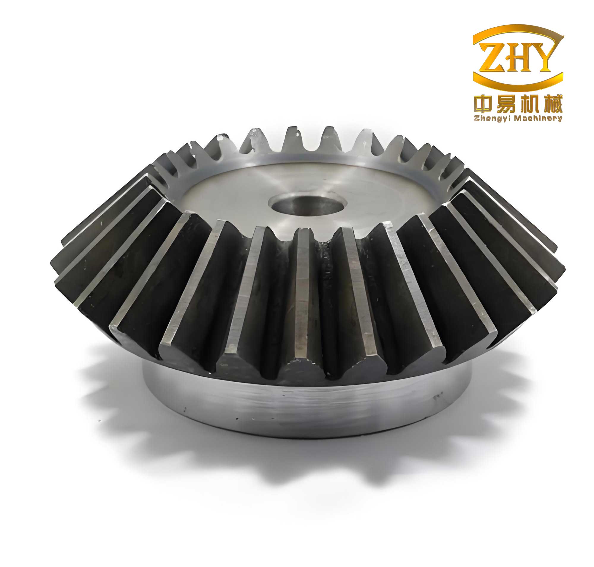
bevel gear sets are distinguished by their conical shape, which allows for smooth engagement between axes that are not parallel. The design and manufacture of these gears are more complex than those of parallel-axis spur or helical gears, but their utility in applications like automotive differentials, industrial machinery, and aerospace actuators is indispensable. Key characteristics driving their selection include high load-bearing capacity, durability, and the ability to provide right-angle drives in a relatively confined space. The optimization of a bevel gear transmission, therefore, targets not just performance but also the minimization of space claim and weight—critical factors in modern machinery. The core of any optimization problem lies in the formulation of a valid mathematical model that accurately represents the physical system and its constraints.
Mathematical Modeling for bevel gear Optimization
The first step in optimizing a 90-degree straight bevel gear pair is to define the design variables. For our purpose, we select the module, the pinion tooth number, and the face width coefficient, as these directly govern the gear’s size and strength.
$$ \mathbf{x} = [x_1, x_2, x_3]^T = [m, z_1, \phi_R]^T $$
Where:
- $m$ is the module of the bevel gear.
- $z_1$ is the number of teeth on the pinion (smaller gear).
- $\phi_R$ is the face width coefficient, defined as the ratio of the face width $b$ to the outer cone distance $R$ ($\phi_R = b/R$).
The number of teeth on the gear ($z_2$) is derived from the fixed transmission ratio $u$, where $u = z_2 / z_1$.
Objective Function: Volume Minimization
The primary goal is to minimize the material volume of the gear pair, approximated by the sum of the volumes of their conical pitch bodies. A simplified and effective objective function for the combined volume is given by:
$$ f(\mathbf{x}) = \frac{\pi}{8} m^3 z_1^3 \phi_R (1 – \phi_R + \frac{\phi_R^2}{3}) \times u(1+u) $$
Substituting the design variables, the function to be minimized becomes:
$$ f(\mathbf{x}) = \frac{\pi}{8} \times u \times (1+u) \times x_1^3 \times x_2^3 \times x_3 \times (1 – x_3 + \frac{x_3^2}{3}) $$
For a fixed ratio $u$, minimizing $f(\mathbf{x})$ directly leads to a more compact bevel gear drive.
Constraint Formulation
The design must satisfy a set of geometric, kinematic, and strength constraints to ensure proper function, prevent failure, and adhere to manufacturing guidelines.
1. Geometric and Manufacturing Constraints:
- Module Bound: The module must be positive and is practically limited by available tooling and size requirements.
$$ g_1(\mathbf{x}) = 2.0 – x_1 \le 0 $$
(Assuming an upper bound of 2 mm for this specific case). - Undercutting Prevention: The pinion must have sufficient teeth to avoid interference during generation. For a 90-degree bevel gear with a standard pressure angle, a practical limit is:
$$ g_2(\mathbf{x}) = \frac{17}{\sqrt{u^2 + 1}} – x_2 \le 0 \quad \text{or equivalently} \quad x_2 \ge \frac{17}{\sqrt{u^2 + 1}} $$ - Face Width Coefficient: For structural rigidity and proper load distribution, $\phi_R$ is typically constrained.
$$ g_3(\mathbf{x}) = 0.3 – x_3 \le 0 $$
$$ g_4(\mathbf{x}) = x_3 – 0.2 \le 0 $$
This bounds $\phi_R$ between 0.2 and 0.3.
2. Strength Constraints (Contact and Bending): These are critical for the bevel gear‘s durability. They ensure the gears can withstand the operational loads without pitting (surface fatigue) or tooth breakage (bending fatigue).
- Contact Stress Constraint: Based on the AGMA or similar standard, the contact stress $\sigma_H$ must not exceed the allowable stress $[\sigma_H]$. The constraint is derived from the pinion’s pitch diameter $d_1 = m z_1$.
$$ \sigma_H = Z_E \sqrt{ \frac{2 K T_1}{\phi_R (1-0.5\phi_R)^2 d_1^3} \cdot \frac{u+1}{u} } \le [\sigma_H] $$
Rearranging to a standard form for the optimization model:
$$ g_5(\mathbf{x}) = \frac{2.92^3 Z_E^2 K T_1}{\phi_R (1-0.5\phi_R)^2 d_1^3 u} – [\sigma_H]^2 \le 0 $$
In terms of design variables:
$$ g_5(\mathbf{x}) = \frac{2.92^3 Z_E^2 K T_1}{x_3 (1-0.5x_3)^2 (x_1 x_2)^3 u} – [\sigma_H]^2 \le 0 $$ - Bending Stress Constraint (Pinion and Gear): The bending stress $\sigma_F$ at the tooth root must be below the allowable bending stress $[\sigma_F]$. Separate constraints are needed for the pinion and gear due to potentially different materials and tooth shapes (via the form factor $Y_{Fa}$ and stress correction factor $Y_{Sa}$).
$$ \sigma_F = \frac{4 K T_1 Y_{Fa} Y_{Sa}}{\phi_R (1-0.5\phi_R)^2 m^3 z_1^2 \sqrt{u^2+1}} \le [\sigma_F] $$
For the pinion:
$$ g_6(\mathbf{x}) = \frac{4 K T_1 (Y_{Fa} Y_{Sa})_1}{x_3 (1-0.5x_3)^2 x_1^3 x_2^2 \sqrt{u^2+1}} – [\sigma_F]_1 \le 0 $$
For the gear, the torque is scaled by the ratio, and the tooth form factors differ:
$$ g_7(\mathbf{x}) = \frac{4 K T_1 (Y_{Fa} Y_{Sa})_2}{x_3 (1-0.5x_3)^2 x_1^3 x_2^2 \sqrt{u^2+1}} \cdot \frac{1}{u} – [\sigma_F]_2 \le 0 $$
The complete Nonlinear Programming (NLP) problem for the bevel gear optimization is therefore:
$$
\begin{aligned}
& \underset{\mathbf{x}}{\text{minimize}}
& & f(\mathbf{x}) = \frac{\pi}{8} u (1+u) x_1^3 x_2^3 x_3 (1 – x_3 + \frac{x_3^2}{3}) \\
& \text{subject to}
& & g_i(\mathbf{x}) \le 0, \quad i = 1, 2, …, 7 \\
& & & \mathbf{x} = [m, z_1, \phi_R]^T > 0
\end{aligned}
$$
Computational Implementation Using MATLAB
Solving this constrained optimization problem efficiently requires computational power. MATLAB’s Optimization Toolbox provides robust algorithms suitable for this task. The `fmincon` function is ideal for solving constrained nonlinear minimization problems. The implementation involves creating three key components: the objective function, the nonlinear constraint function, and the main calling script.
The core of the algorithm involves the sequential quadratic programming (SQP) method, which iteratively solves quadratic approximations of the original problem. The following table summarizes the key parameters and material properties used in our specific case study:
| Parameter | Symbol | Value | Unit |
|---|---|---|---|
| Transmission Ratio | $u$ | 5 | – |
| Input Torque | $T_1$ | 182 | Nm |
| Pinion Material | – | 20CrMnTi (Case-hardened) | – |
| Gear Material | – | 40Cr (Heat-treated) | – |
| Allowable Contact Stress | $[\sigma_H]$ | 1350 | MPa |
| Allowable Bending Stress (Pinion) | $[\sigma_F]_1$ | 657 | MPa |
| Allowable Bending Stress (Gear) | $[\sigma_F]_2$ | 263 | MPa |
| Elastic Coefficient | $Z_E$ | 189.8 | $\sqrt{\text{MPa}}$ |
| Application Factor | $K$ | 1.25 | – |
| Form Factor (Pinion) | $Y_{Fa1}$ | 2.85 | – |
| Stress Correction Factor (Pinion) | $Y_{Sa1}$ | 1.54 | – |
| Form Factor (Gear) | $Y_{Fa2}$ | 2.25 | – |
| Stress Correction Factor (Gear) | $Y_{Sa2}$ | 1.85 | – |
The objective function is coded in a file `objfun.m`:
function f = objfun(x)
    u = 5;
    f = (pi/8) * u * (1+u) * x(1)^3 * x(2)^3 * x(3) * (1 - x(3) + x(3)^2/3);
end
The nonlinear constraints are coded in `confun.m`. Note that the inequalities are structured in the form $c(\mathbf{x}) \le 0$ as required by `fmincon`.
function [c, ceq] = confun(x)
    u = 5; T1 = 182; K = 1.25; ZE = 189.8;
    sigma_H_all = 1350^2; % Squared for constraint form
    sigma_F1_all = 657; sigma_F2_all = 263;
    YFaSa1 = 2.85 * 1.54; YFaSa2 = 2.25 * 1.85;

    % Initialize constraints
    c = zeros(7,1);

    % g1: Module upper bound
    c(1) = 2.0 - x(1);
    % g2: Minimum pinion teeth (rearranged to c <= 0 form)
    c(2) = 17/sqrt(u^2+1) - x(2);
    % g3: Face width coefficient upper bound
    c(3) = x(3) - 0.3; % Note: Our g3 was 0.3 - x3 <= 0 => c = x3 - 0.3
    % g4: Face width coefficient lower bound
    c(4) = 0.2 - x(3); % Our g4 was x3 - 0.2 >= 0 => 0.2 - x3 <= 0
    % g5: Contact stress constraint
    d1 = x(1) * x(2);
    c(5) = ( (2.92^3 * ZE^2 * K * T1) / (x(3) * (1-0.5*x(3))^2 * d1^3 * u) ) - sigma_H_all;
    % g6: Bending stress constraint for pinion
    c(6) = ( (4 * K * T1 * YFaSa1) / (x(3) * (1-0.5*x(3))^2 * x(1)^3 * x(2)^2 * sqrt(u^2+1)) ) - sigma_F1_all;
    % g7: Bending stress constraint for gear
    c(7) = ( (4 * K * T1 * YFaSa2) / (x(3) * (1-0.5*x(3))^2 * x(1)^3 * x(2)^2 * sqrt(u^2+1)) ) * (1/u) - sigma_F2_all;

    % No equality constraints
    ceq = [];
end
The main script sets the initial guess (an initial feasible design) and calls the solver. The choice of initial point can influence convergence speed but not the final optimal solution in a convex problem region.
x0 = [4; 15; 0.3]; % Initial guess [m, z1, phi_R]
options = optimoptions('fmincon', 'Display', 'iter', 'Algorithm', 'sqp');
[x_opt, fval_opt] = fmincon(@objfun, x0, [], [], [], [], [], [], @confun, options);
The solver iteratively evaluates the objective and constraints, adjusting the design variables until it finds a local minimum that satisfies all constraints. The final output provides the optimal set of parameters.
Results, Analysis, and Practical Significance
Executing the optimization routine yields a significant improvement over an initial, intuitively chosen design. The optimal design parameters and a comparison with the initial guess are presented below.
| Design Variable / Metric | Initial Design | Optimal Design | Unit | Change |
|---|---|---|---|---|
| Module, $m$ | 4.0 | 3.5 | mm | -12.5% |
| Pinion Teeth, $z_1$ | 15 | 15 | – | 0% |
| Face Width Coeff., $\phi_R$ | 0.3 | 0.3 | – | 0% |
| Gear Teeth, $z_2 = u \cdot z_1$ | 75 | 75 | – | 0% |
| Pitch Diameter (Pinion), $d_1 = m z_1$ | 60.0 | 52.5 | mm | -12.5% |
| Outer Cone Distance, $R$ | 94.9 | 83.0 | mm | -12.5% |
| Approximate Gear Pair Volume | ~69,626,000 | ~46,644,000 | mm³ | -33.0% |
The results are striking. The optimization algorithm successfully reduced the module from 4 mm to 3.5 mm while keeping the number of teeth constant. This reduction directly decreases the pitch diameters and the overall cone distance $R$. Since all linear dimensions scale with the module, the volume, which is a cubic function of these dimensions, experiences a dramatic reduction of approximately 33%. This is a substantial saving in material, weight, and occupied space.
It is crucial to analyze why the optimizer converged to this point. The lower bound for the pinion tooth count ($g_2$) and the upper bound for the face width coefficient ($g_3$) were active constraints, meaning the optimal solution lies precisely at these boundaries: $z_1 = 17/\sqrt{26} \approx 15$ and $\phi_R = 0.3$. This indicates that to minimize volume, the design is pushed to use the smallest permissible pinion (reducing $d_1$) and the widest permissible face (allowing a smaller diameter for the same bending/contact capacity). The module was then reduced until the most critical strength constraint (likely the bending stress on the gear, given its lower allowable stress $[\sigma_F]_2$) became active. The initial design was over-engineered, with a larger module providing unnecessary safety margins at the cost of size and weight.
The broader implications for bevel gear design are profound. This mathematical optimization approach moves the process from one based on handbook recommendations and safety factors to a precise, performance-driven calculation. It enables engineers to:
- Achieve Minimum Weight: Critical in aerospace, automotive, and robotics.
- Reduce Material Cost: Direct savings from using less metal or advanced material.
- Improve System Integration: A smaller bevel gear housing allows for more compact machinery layouts.
- Enhance Dynamic Performance: Lower inertia from smaller gears can lead to faster system response.
Furthermore, the model is adaptable. The objective function could be changed to minimize power loss (maximize efficiency) or to minimize a cost function that includes manufacturing expenses. Additional constraints, such as specific center distance requirements, limits on gear ratio deviation, or reliability-based probabilistic constraints, can be incorporated into the same framework.
In conclusion, the application of nonlinear programming techniques to the design of a bevel gear transmission provides a rigorous and highly effective methodology for achieving optimal performance. By formulating the physical design problem as a mathematical model with a clear objective (volume minimization) and realistic constraints (strength and geometry), and by leveraging computational solvers like those in MATLAB, engineers can systematically discover designs that are significantly superior to those obtained through traditional iterative or handbook methods. This case study demonstrates a 33% reduction in estimated volume, underscoring the potential of optimization to drive innovation and efficiency in mechanical power transmission systems employing bevel gears.