
The operational integrity of helicopter transmission systems is paramount to flight safety and mission capability. At the heart of the main reducer, serving as the critical power input interface, lies the bevel gear train. Bevel gears enable the efficient transmission of power between intersecting axes, a fundamental requirement in helicopter drivetrains. Their design offers high load capacity and reliability. However, constrained by stringent weight and spatial considerations, helicopter transmissions often adopt non-redundant series configurations. This, coupled with the demanding operational envelopes involving high speeds, heavy loads, and constantly varying flight conditions, renders bevel gears susceptible to fatigue-induced failures. The complex, coupled multi-degree-of-freedom dynamics inherent to bevel gear meshing further complicate the understanding of their behavior under fault conditions. Therefore, developing a high-fidelity dynamic model capable of simulating both healthy and damaged states is crucial for elucidating fault mechanisms, enabling early damage detection, and ultimately supporting the development of robust Health and Usage Monitoring Systems (HUMS). This article presents a comprehensive nonlinear dynamic modeling approach for a helicopter main reducer bevel gear system, featuring an innovative method for calculating time-varying mesh stiffness and an analysis of the dynamic response to gear tooth faults.
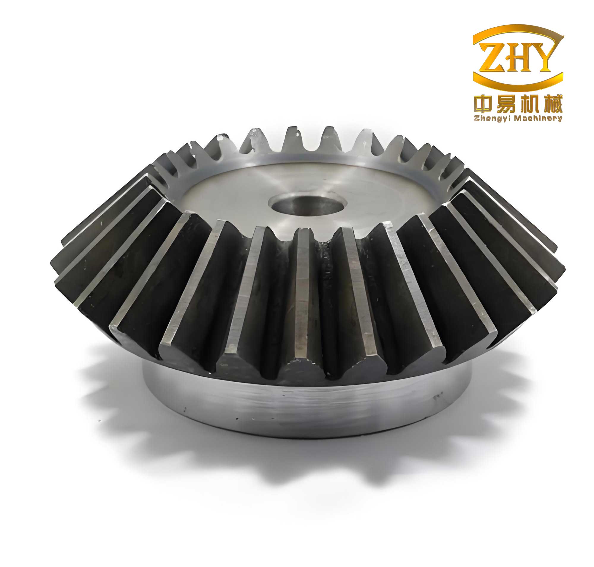
1. Nonlinear Dynamic Modeling of the Bevel Gear System
The first step towards analyzing system response is establishing an accurate dynamic model. A lumped-parameter approach is employed to model the helical bevel gear pair. The system is simplified into two rigid cones, representing the pinion and the gear, connected by a nonlinear spring-damper element that models the gear mesh interface. The model accounts for eight degrees of freedom (DOFs): lateral (x), longitudinal (y), and axial (z) translations, and torsional rotation (θ) for both the pinion and gear. Key internal excitations such as time-varying mesh stiffness, transmission error, and backlash are incorporated. The model is formulated as a bending-torsion-axial coupled system.
To derive the equations of motion, the conical bevel gears are first transformed into equivalent spur gears for ease of analyzing the mesh action along the line of contact. The dynamic transmission error (DTE), which is the primary source of vibration, is defined along this line of action. For a bevel gear pair, the DTE, denoted by λ, is a function of the translational and rotational displacements of both gears, modified by their cone angles.
Let δ₁ and δ₂ be the pitch cone angles of the pinion and gear, respectively. The coordinates of the equivalent model (x_e, z_e) relate to the physical model coordinates (x, z) through the cone angles. The relationships for the pinion are:
$$ x_{e1} = x_1 \cos\delta_1 + z_1 \sin\delta_1 $$
$$ z_{e1} = -x_1 \sin\delta_1 + z_1 \cos\delta_1 $$
And for the gear:
$$ x_{e2} = x_2 \cos\delta_2 – z_2 \sin\delta_2 $$
$$ z_{e2} = x_2 \sin\delta_2 + z_2 \cos\delta_2 $$
The rotational displacement contribution is proportional to the base circle radius R. Therefore, the complete expression for the dynamic transmission error λ becomes:
$$ \lambda = (x_1 \sin\alpha \cos\delta_1 + y_1 \cos\alpha + z_1 \sin\alpha \sin\delta_1 + R_1\theta_1) – (x_2 \sin\alpha \cos\delta_2 + y_2 \cos\alpha – z_2 \sin\alpha \sin\delta_2 + R_2\theta_2) – e(t) $$
where α is the pressure angle, and e(t) is the static transmission error.
The nonlinear mesh force F_m is then formulated as a combination of the elastic force from the time-varying mesh stiffness k_m(t) and the damping force proportional to the velocity of the DTE. A clearance function f(λ) accounts for tooth backlash 2b.
$$ F_m = k_m(t) f(\lambda) + c_m \dot{\lambda} $$
$$ f(\lambda) = \begin{cases}
\lambda – b, & \lambda > b \\
0, & |\lambda| \le b \\
\lambda + b, & \lambda < -b
\end{cases} $$
Applying Newton’s second law to each DOF yields the complete set of nonlinear differential equations for the 8-DOF bevel gear system. The equations for the pinion are shown below as an example. The equations for the gear are symmetric, considering the opposite direction of the mesh force.
Pinion Equations:
$$ m_1 \ddot{x}_1 + c_m \dot{\lambda} \sin\alpha \cos\delta_1 + k_m(t) f(\lambda) \sin\alpha \cos\delta_1 + c_{bx1} \dot{x}_1 + k_{bx1} x_1 = 0 $$
$$ m_1 \ddot{y}_1 + c_m \dot{\lambda} \cos\alpha + k_m(t) f(\lambda) \cos\alpha + c_{by1} \dot{y}_1 + k_{by1} y_1 = 0 $$
$$ m_1 \ddot{z}_1 + c_m \dot{\lambda} \sin\alpha \sin\delta_1 + k_m(t) f(\lambda) \sin\alpha \sin\delta_1 + c_{bz1} \dot{z}_1 + k_{bz1} z_1 = 0 $$
$$ J_1 \ddot{\theta}_1 + c_m \dot{\lambda} R_1 + k_m(t) f(\lambda) R_1 = T_1 $$
Here, m is mass, J is polar mass moment of inertia, c_b and k_b are bearing damping and stiffness, and T is external torque.
2. A Novel “Slicing Method” for Bevel Gear Mesh Stiffness
The time-varying mesh stiffness k_m(t) is a critical parameter in the dynamic model. For spur or helical cylindrical gears, the potential energy method is well-established. However, its direct application to bevel gears is limited due to the tapered tooth geometry, where the tooth profile and module vary continuously along the face width. To overcome this, an innovative “slicing method” is proposed for calculating the mesh stiffness of straight bevel gear pairs.
The core idea is to discretize the tooth of the bevel gear into a finite number (n) of thin slices along the face width L. Each slice, with a thickness dl, can be approximated as a spur gear tooth with constant dimensions at that specific section. By calculating the “local” or “slice” stiffness for each segment and summing them along the face width, the total mesh stiffness of the bevel gear pair is obtained.
$$ k_{total}(t) = \sum_{i=1}^{n} k_{slice}^i(t) $$
The process involves calculating the equivalent spur gear parameters for each slice. Key geometric parameters like the reference cone distance R_zj, module m_r, and addendum h_ar are determined at the mid-point of each slice. These are then used to derive the equivalent spur gear parameters: equivalent number of teeth Z_v, equivalent pitch diameter d_vr, equivalent base circle diameter d_vbr, etc.
Once the equivalent spur gear parameters for a slice are known, the potential energy method is applied to calculate the stiffness components for that slice. For a healthy tooth, the total compliance of a single slice in a meshing pair is the sum of Hertzian contact compliance, bending, shear, axial compressive compliances, and the fillet foundation compliance for both the pinion and gear teeth.
$$ \frac{1}{k_{slice}} = \frac{1}{k_h} + \sum_{j=1}^{2}\left( \frac{1}{k_{b,j}} + \frac{1}{k_{a,j}} + \frac{1}{k_{s,j}} + \frac{1}{k_{f,j}} \right) $$
Where subscripts b, a, s, f, and h denote bending, axial, shear, foundation, and Hertzian contact stiffness, respectively. The formulas for these compliances, expressed in terms of the slice’s geometric parameters and material properties (Young’s modulus E, Poisson’s ratio ν), are evaluated via integration along the tooth profile. For the bending compliance of a healthy tooth slice, as an example, the integral covers both the fillet and involute regions:
$$ \frac{1}{k_b} = \int_{0}^{d_1} \frac{3[(\alpha_2 – \alpha) \cos\alpha]^2}{2E(dl)[\sin\alpha + (\alpha_2 – \alpha)\cos\alpha]^3} d\alpha + \text{(integral for fillet region)} $$
Modeling Crack Faults: To simulate a root crack, it is modeled as a straight line starting from the fillet curve at an angle γ and propagating inward by a length q. The crack affects the effective area and moment of inertia of the tooth cross-section within the cracked zone. This primarily alters the bending and shear stiffness calculations. The cross-sectional area A_x and area moment of inertia I_x for a cracked segment become:
$$ dA_x = (h_c + h_x) dl \quad \text{for} \quad x \le d_c $$
$$ dI_x = \frac{1}{12}(h_c + h_x)^3 dl \quad \text{for} \quad x \le d_c $$
Where h_c is the residual tooth thickness at the crack tip and d_c is the distance from the crack start point to the tooth centerline. These modified expressions are substituted into the integrals for bending and shear compliances, changing the integration limits and the integrand’s denominator in the cracked region. The other stiffness components (axial, Hertzian, foundation) are assumed unaffected by a root crack. The compliance for a cracked slice is thus:
$$ \frac{1}{k_{slice,crack}} = \frac{1}{k_h} + \left( \frac{1}{k_{b1,crack}} + \frac{1}{k_{a1}} + \frac{1}{k_{s1,crack}} + \frac{1}{k_{f1}} \right) + \left( \frac{1}{k_{b2}} + \frac{1}{k_{a2}} + \frac{1}{k_{s2}} + \frac{1}{k_{f2}} \right) $$
This method allows for efficient and accurate evaluation of the time-varying mesh stiffness for both healthy and cracked bevel gears, providing the essential input for the nonlinear dynamic model.
3. Simulation Results and Dynamic Response Analysis
The proposed models are applied to a case study of a helicopter main reducer bevel gear pair. The basic system parameters are listed in the table below.
| Parameter | Pinion | Gear |
|---|---|---|
| Number of Teeth (Z) | 18 | 36 |
| Module (m_d) [mm] | 4.25 | 4.25 |
| Pressure Angle (α) [deg] | 20 | 20 |
| Face Width (L) [mm] | 27.66 | 27.66 |
| Mass (m) [kg] | 1.313 | 3.679 |
| Polar Moment of Inertia (J) [kg·m²] | 8.270e-4 | 7.340e-3 |
The bearing support stiffness and damping are in the order of 10^8 N/m and 10^3 N·s/m, respectively. A constant pinion speed of 300 rpm (5 Hz) and a gear load torque of 32 N·m are used for simulation. The mesh frequency f_m is 90 Hz.
3.1 Time-Varying Mesh Stiffness under Different Fault States
The slicing method (with n=100 slices) is used to compute k_m(t) for one complete mesh cycle. Seven states are analyzed: healthy, and six cracked pinion states with crack lengths q ranging from 0.5 mm to a complete tooth breakage (simulated by a very deep crack). The results demonstrate that the mesh stiffness waveform for the healthy bevel gear resembles that of a spur gear but accounts for the tapered tooth engagement. As the crack propagates, the mesh stiffness decreases. The reduction is more pronounced in the double-tooth contact regions and becomes progressively larger as the meshing point moves towards the tooth tip (where the bending moment arm is longer). In the case of a broken tooth, the stiffness during the double-tooth contact period where the faulty tooth is engaged drops significantly, and the single-tooth contact stiffness for that tooth pair effectively vanishes.
3.2 Dynamic Response and Fault Feature Evolution
The computed k_m(t) for each fault state is fed into the 8-DOF dynamic model. The equations are solved numerically to obtain the vibration response, particularly the pinion center acceleration in the longitudinal direction (ÿ₁). The analysis focuses on the evolution of time-domain and frequency-domain features with increasing crack severity.
Time-Domain Analysis: The healthy state exhibits a simple periodic motion. For small crack lengths (q < 1.5 mm), the time-domain signal shows little visible change, making early fault detection challenging from time waveforms alone. When the crack length reaches 1.5 mm, distinct periodic impulses appear in the acceleration signal. The time interval between these impulses Δt is 0.2 seconds, corresponding precisely to the pinion rotation period (1/5 Hz). This confirms the impulse is generated once per revolution of the faulty pinion. For larger cracks (q = 2.5 mm) and the broken tooth state, these periodic impulses become very pronounced.
Frequency-Domain Analysis: The healthy state spectrum is dominated by the mesh frequency f_m and its higher harmonics (2f_m, 3f_m,…). With the introduction and growth of a crack, sidebands emerge around the mesh frequency harmonics. Their amplitude increases with crack severity. The sideband spacing is equal to the pinion rotational frequency f_p (5 Hz). For instance, around the 5th mesh harmonic (5f_m = 450 Hz), prominent sidebands appear at 450 ± 5 Hz, 450 ± 10 Hz, etc. This modulation is a classic signature of a localized gear fault. The table below summarizes the observed features.
| Fault State | Time-Domain Feature | Frequency-Domain Feature |
|---|---|---|
| Healthy / Small Crack (q<1.5mm) | Periodic, no clear impulses | Mesh harmonics dominant; very low sidebands. |
| Medium Crack (q=1.5mm) | Visible periodic impulses at T_p (0.2s). | Sidebands at f_m ± k·f_p appear; amplitude increases. |
| Severe Crack / Broken Tooth | Large, distinct periodic impulses. | Sideband amplitudes are significantly elevated. |
The simulation results clearly illustrate the mechanism by which a tooth root crack in a bevel gear modifies the system dynamics: it reduces the local mesh stiffness, which in turn modulates the vibration signal at the fault frequency, generating identifiable sidebands in the spectrum. The model successfully captures the progression of these fault features.
4. Experimental Validation
To validate the dynamic model and the fault response analysis, experimental tests were conducted on a dedicated helicopter transmission diagnostic test bench. The setup includes a drive motor, the bevel gear stage, subsequent planetary gear stages, and a load motor. For conclusive validation, a broken tooth fault was introduced on the pinion using wire-cut electrical discharge machining (EDM).
| Test Object | State | Pinion Speed [rpm] | Gear Load [N·m] |
|---|---|---|---|
| Bevel Gear Stage | Baseline (Healthy) | 300 | 82.4 |
| Bevel Gear Stage | Pinion Broken Tooth | 300 | 82.4 |
Vibration acceleration data was acquired from a sensor mounted on the pinion housing. The time-domain signals for the healthy and faulty states are distinctly different. The healthy state signal shows relatively steady vibration. In contrast, the broken tooth state signal exhibits strong periodic impulses with an interval of 0.2 seconds, matching the pinion’s rotational period and the simulation predictions.
Frequency-domain analysis using power spectral density (PSD) further confirms the findings. The healthy baseline spectrum shows mesh harmonics with minimal sideband activity. The broken tooth spectrum retains the mesh harmonics but now exhibits prominent sidebands around these harmonics (e.g., around f_m and 3f_m). The sideband spacing is 5 Hz, exactly the pinion rotational frequency f_p. The amplitude of these fault-induced sidebands is significantly higher in the broken tooth case compared to the baseline. These experimental observations—periodic impulses in the time domain and increased sideband activity in the frequency domain—align perfectly with the characteristics predicted by the nonlinear dynamic model for a severe bevel gear tooth fault. This consistency validates the accuracy and effectiveness of the proposed modeling framework.
5. Conclusion
This work has developed a comprehensive framework for the dynamic analysis of helicopter main reducer bevel gear systems under health and fault conditions. The key contributions are threefold. First, a nonlinear, bending-torsion-axial coupled dynamic model for a bevel gear pair was established using the lumped-parameter method, incorporating essential nonlinearities like time-varying mesh stiffness and backlash. Second, an innovative “slicing method” was proposed to calculate the time-varying mesh stiffness of straight bevel gear pairs. This method effectively overcomes the limitation of traditional potential energy methods by discretizing the tapered tooth, enabling efficient and accurate stiffness evaluation for both healthy and cracked bevel gears. Third, through integrated simulation and experimental testing, the model’s capability to simulate dynamic responses and reveal fault mechanisms was demonstrated. The results show that as a root crack propagates in a bevel gear, the mesh stiffness degrades, leading to periodic impulses in the time-domain response and characteristic sidebands around mesh harmonics in the frequency domain. The spacing of these features correlates with the faulty gear’s rotational speed. The close agreement between simulation and experimental results confirms the model’s validity. This modeling and analysis framework provides a solid theoretical foundation and a valuable simulation tool for understanding bevel gear dynamics, guiding the design of more robust transmissions, and developing advanced fault diagnosis algorithms for helicopter Health and Usage Monitoring Systems.