
The evolution of mechanical design has progressively shifted from deterministic methods towards probabilistic approaches to better account for the inherent uncertainties in material properties, manufacturing tolerances, and operational loads. Reliability design, also known as probabilistic design, represents this modern paradigm. It fundamentally differs from conventional design by treating key parameters not as fixed values but as random variables governed by statistical distributions. This article delves into the core theories of mechanical reliability design and demonstrates its superior application in the design and analysis of a critical component: the gear shaft.
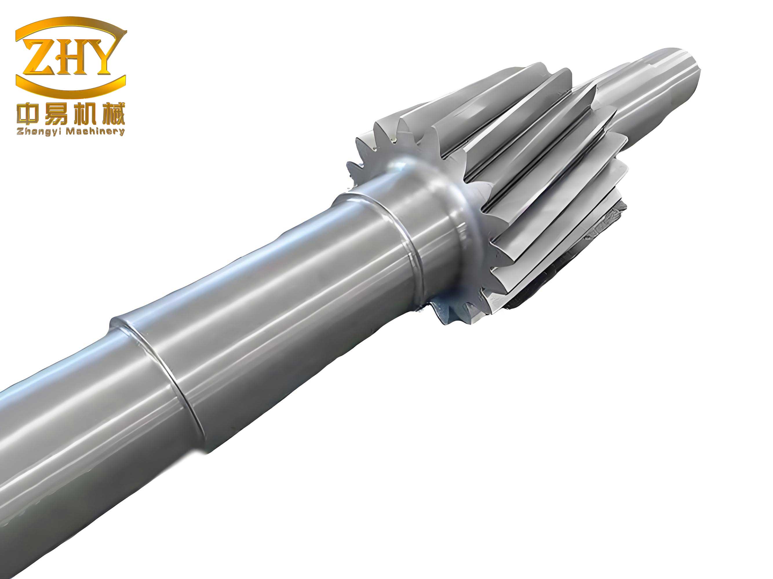
The traditional safety factor method, while simple, often leads to overly conservative or, in some cases, inadequately safe designs because it ignores variability. A safety factor of 2 does not guarantee zero failures if the scatter in strength and stress is high. Reliability design, in contrast, quantifies risk. It allows an engineer to explicitly define and achieve a target probability of success (reliability) or an acceptable probability of failure. For components like a gear shaft, which transmits power and moments in demanding conditions, this methodology is crucial for optimizing weight, cost, and performance while ensuring operational integrity.
Core Theory: The Stress-Strength Interference Model
The foundational concept of reliability design is the Stress-Strength Interference (SSI) theory. It posits that both the component’s strength (S) and the applied stress (L) are random variables with their own probability density functions (PDFs), denoted as $f_S(s)$ and $g_L(l)$, respectively. Failure occurs when the applied stress exceeds the component’s strength. The probability of this event is the failure probability ($P_f$), and the reliability ($R$) is the probability that strength exceeds stress.
$$ R = P(S > L) = P[(S – L) > 0] $$
$$ P_f = P(L > S) = 1 – R $$
Graphically, these two distributions are plotted on the same axis. The region where they overlap or “interfere” represents the potential for failure. The reliability is not simply the area under the strength curve to the right of a single stress value, but the integrated probability over all possible stress values. Mathematically, for a given stress value $l$, the conditional probability of failure is the probability that strength is less than $l$, which is $F_S(l)$, the cumulative distribution function (CDF) of strength. Integrating this over all possible stresses weighted by the stress PDF gives the total failure probability:
$$ P_f = \int_{-\infty}^{\infty} F_S(l) \cdot g_L(l) \, dl $$
$$ R = 1 – P_f = \int_{-\infty}^{\infty} [1 – F_S(l)] \cdot g_L(l) \, dl = \int_{-\infty}^{\infty} R_S(l) \cdot g_L(l) \, dl $$
This model directly incorporates the randomness of both strength and stress, providing a far more realistic assessment of a component’s safety than a deterministic safety factor. When applying this to a gear shaft, ‘strength’ refers to its fatigue limit or yield strength, while ‘stress’ refers to the combined bending and torsional stresses at the critical cross-section.
Reliability Calculation for Normally Distributed Variables
Extensive empirical data shows that the strength of many materials and the operational loads on components like a gear shaft can often be reasonably modeled by the normal (Gaussian) distribution. This assumption leads to a powerful and simplified formulation for reliability calculation.
Let strength $S \sim N(\mu_S, \sigma_S^2)$ and stress $L \sim N(\mu_L, \sigma_L^2)$, where $\mu$ denotes the mean and $\sigma$ the standard deviation. The safety margin, $Z = S – L$, is also a normally distributed random variable:
$$ Z \sim N(\mu_Z, \sigma_Z^2) $$
$$ \mu_Z = \mu_S – \mu_L $$
$$ \sigma_Z = \sqrt{\sigma_S^2 + \sigma_L^2} $$
The probability of failure is $P_f = P(Z < 0)$. By standardizing the variable, we get the cornerstone of reliability analysis: the Reliability Index ($\beta$) or Link Equation.
$$ \beta = \frac{\mu_Z}{\sigma_Z} = \frac{\mu_S – \mu_L}{\sqrt{\sigma_S^2 + \sigma_L^2}} $$
The reliability is then found from the standard normal CDF, $\Phi(\cdot)$:
$$ R = P(Z > 0) = \Phi(\beta) $$
This equation elegantly links the statistical parameters of stress and strength to the component’s reliability. For a target reliability $R$, one can find the corresponding $\beta$ from standard normal tables and then solve the link equation for the unknown design parameter (e.g., the diameter of the gear shaft). This is the essence of reliability-based design.
| Design Parameter | Symbol | Typical Distribution | Notes for Gear Shaft |
|---|---|---|---|
| Material Yield Strength | $S_y$ | Normal, Weibull | Mean from tests, COV ~ 5-10% |
| Material Fatigue Limit | $S_e$ | Log-normal, Weibull | Highly scattered; depends on surface finish, size. |
| Bending Moment | $M$ | Normal, Extreme Value | Derived from load analysis on gear teeth. |
| Torque | $T$ | Normal | Depends on driven load fluctuations. |
| Stress Concentration Factor | $K_f$ | Deterministic or Random | For keyways, fillets. Can be treated as a random variable to account for manufacturing variance. |
| Diameter | $d$ | Normal (Tolerance) | Manufacturing tolerances define $\sigma_d$. |
Practical Application: Reliability Design of a Gear Shaft
Consider the redesign of a failed gear shaft made of quenched and tempered 40Cr steel. The goal is to determine a new diameter for the critical section with a specified high reliability, addressing the failure mode observed.
1. Problem Definition and Input Parameters
The shaft failed due to fatigue. Load analysis identified a critical section subjected to a fully reversed bending moment $M$ and a repeated (zero-based) torque $T$. The original design used deterministic methods. We now apply reliability design with the following targets and data:
- Target Reliability: $R = 0.99$ ($\beta = 2.326$ from standard normal tables).
- Desired Safety Margin (optional): A mean strength reserve factor $n$ can be initially targeted (e.g., $n=1.25$).
- Load Statistics: Equivalent bending moment $\mu_M = 7500\ Nm$, $\sigma_M = 0.08\mu_M$. Equivalent torque $\mu_T = 7800\ Nm$, $\sigma_T = 0.08\mu_T$. The coefficient of variation (COV) of 0.08 is common for load estimates.
- Strength Statistics (Fatigue): The corrected endurance limit $S_e’$ is random.
$$ \mu_{S_e’} = \frac{0.43 \cdot \mu_{\sigma_b}}{K_f} $$
For 40Cr, $\mu_{\sigma_b} = 735\ MPa$. The fatigue stress concentration factor at the critical fillet or keyway is $K_f = 2.0$. Therefore, $\mu_{S_e’} = 158.0\ MPa$. A typical COV for fatigue strength is 0.08, so $\sigma_{S_e’} = 0.08 \times 158.0 = 12.6\ MPa$.
2. Reliability-Based Design for Diameter
The von Mises stress is used for the combined stress state. For a solid round gear shaft of diameter $d$, the maximum stress is:
$$ \sigma_{max} = \sqrt{ \left( \frac{32 M}{\pi d^3} \right)^2 + 3 \left( \frac{16 T}{\pi d^3} \right)^2 } = \frac{32}{\pi d^3} \sqrt{ M^2 + 0.75 T^2 } $$
The factor 0.75 arises from the distortion energy theory for a repeated torsion versus fully reversed bending. Let $K_M = 32/\pi$ and $\alpha = 0.75$. The stress is:
$$ \sigma = \frac{K_M}{d^3} \sqrt{ M^2 + \alpha T^2 } $$
This is a nonlinear function of random variables $M$, $T$, and $d$. For reliability calculation, we need the mean and standard deviation of stress, $\mu_\sigma$ and $\sigma_\sigma$.
Approximation using Taylor Series Expansion (First Order):
If $X$ and $Y$ are independent, and $Z = \sqrt{X^2 + Y^2}$, approximate formulas exist. However, a more direct approach for design is to assume we want the mean stress $\mu_\sigma$ to equal a target value derived from the reliability equation. We can rearrange the link equation, solving for the required mean stress $\mu_\sigma$ that satisfies the target $\beta$, given the mean and variation of strength.
$$ \beta = \frac{\mu_{S_e’} – n \cdot \mu_{\sigma}}{\sqrt{\sigma_{S_e’}^2 + (C_{\sigma} \cdot n \cdot \mu_{\sigma})^2}} $$
Where $n$ is a central safety factor applied to the mean stress, and $C_{\sigma}$ is the coefficient of variation of the stress (e.g., 0.08). Solving for $\mu_\sigma$:
$$ \mu_{\sigma} = \frac{\mu_{S_e’}}{n + \beta \sqrt{ \left(\frac{\sigma_{S_e’}}{\mu_{S_e’}}\right)^2 + C_{\sigma}^2 } } $$
Substituting our values: $\mu_{S_e’}=158.0\ MPa$, $\sigma_{S_e’}=12.6\ MPa$, $n=1.25$, $\beta=2.326$, $C_{\sigma}=0.08$.
$$ \mu_{\sigma} \approx \frac{158.0}{1.25 + 2.326 \times \sqrt{0.08^2 + 0.08^2}} = \frac{158.0}{1.25 + 2.326 \times 0.1131} \approx 98.9\ MPa $$
Now, equate this mean stress to the stress formula using mean loads:
$$ \mu_{\sigma} = \frac{K_M}{\mu_d^3} \sqrt{ \mu_M^2 + \alpha \mu_T^2 } $$
Solve for the mean diameter $\mu_d$:
$$ \mu_d = \left( \frac{K_M}{\mu_{\sigma}} \sqrt{ \mu_M^2 + \alpha \mu_T^2 } \right)^{1/3} $$
$$ \mu_d = \left( \frac{32/\pi}{98.9 \times 10^6} \sqrt{ (7500)^2 + 0.75 \times (7800)^2 } \right)^{1/3} \approx 0.0993\ m = 99.3\ mm $$
Therefore, a gear shaft with a nominal critical diameter of **100 mm** is required to meet the 99% reliability target under the given fatigue loading.
| Design Phase | Parameter | Symbol | Value | Notes |
|---|---|---|---|---|
| Target & Input | Reliability | $R$ | 0.99 | Design requirement. |
| Reliability Index | $\beta$ | 2.326 | From $\Phi^{-1}(0.99)$. | |
| Fatigue Strength Mean | $\mu_{S_e’}$ | 158.0 MPa | Corrected for stress concentration. | |
| Calculation | Allowable Mean Stress | $\mu_{\sigma}$ | 98.9 MPa | Derived from link equation. |
| Required Mean Diameter | $\mu_d$ | 99.3 mm | From stress equation. | |
| Output | Final Nominal Diameter | $d$ | 100 mm | Rounded up to standard size. |
3. Discussion and Sensitivity
This process highlights key advantages. The traditional design might have simply used mean loads and a safety factor on a deterministic endurance limit, likely resulting in a different diameter. The reliability method quantitatively accounts for:
1. Scatter in Material Fatigue Strength: The 8% COV on $S_e’$ directly influences $\beta$.
2. Load Variation: The 8% COV on $M$ and $T$ is factored into the stress variation $C_{\sigma}$.
3. Explicit Risk Target: The design meets a specific, quantifiable reliability goal, not an ambiguous “safe” condition.
A sensitivity analysis can be performed by observing the partial derivatives in the link equation. The reliability of the gear shaft is most sensitive to parameters with the largest normalized gradients. For instance, improving manufacturing quality to reduce the stress concentration factor $K_f$ from 2.0 to 1.8 would increase $\mu_{S_e’}$ significantly, thereby greatly enhancing reliability or allowing a smaller diameter for the same reliability.
Advanced Considerations and System Reliability
The preceding analysis assumes normal distributions for simplicity. In practice, other distributions like the Weibull distribution (excellent for fatigue life and strength) or the log-normal distribution (for strictly positive data) may be more appropriate. The fundamental SSI theory still applies, but the reliability integral $R = \int F_S(l) g_L(l) dl$ may require numerical integration or simulation techniques like Monte Carlo Simulation (MCS).
$$ \text{MCS Algorithm:} $$
$$ 1. \ \text{Generate random sample } s_i \text{ from } f_S(s) $$
$$ 2. \ \text{Generate random sample } l_i \text{ from } g_L(l) $$
$$ 3. \ \text{Count failure if } l_i > s_i $$
$$ 4. \ \text{Repeat } N \text{ times. } \hat{P}_f = \frac{N_{fail}}{N}, \ \hat{R} = 1 – \hat{P}_f $$
Furthermore, a gear shaft is part of a larger system (bearings, gears, couplings). System reliability analysis becomes vital. For a series system (where failure of any component fails the system), the system reliability $R_{sys}$ is the product of component reliabilities $R_i$.
$$ R_{sys} = \prod_{i=1}^{n} R_i $$
If the gear shaft has $R_{shaft}=0.99$, but it is in series with a bearing with $R_{bearing}=0.995$, and a coupling with $R_{coupling}=0.997$, the subsystem reliability is:
$$ R_{sub} = 0.99 \times 0.995 \times 0.997 \approx 0.982 $$
This demonstrates how high component reliabilities are needed to achieve acceptable system-level performance. Parallel redundancy can be incorporated for critical components using different formulas.
Design Process Flowchart for a Reliable Gear Shaft
A structured process ensures a comprehensive reliability-based design.
- Define Function and Failure Modes: The gear shaft transmits torque and supports gears. Failure modes include fatigue fracture (dominant), excessive deflection, yield.
- Identify Critical Loads and Stresses: Determine bending moments and torques. Select critical sections (e.g., at stress concentrators).
- Characterize Random Variables: Define statistical models (distribution type, mean, std dev) for:
- Material properties (yield $\sigma_y$, ultimate $\sigma_u$, endurance limit $S_e$).
- Loads (bending moment $M$, torque $T$).
- Geometric dimensions (diameter $d$, tolerance).
- Model uncertainties (stress calculation error).
- Establish Target Reliability ($R_{target}$): Based on safety, cost, consequence of failure. Obtain corresponding $\beta_{target}$.
- Formulate Limit State Function (LSF): The failure boundary. For fatigue of a gear shaft:
$$ g(\mathbf{X}) = S_e’ – \sigma_{max}(M, T, d, …) $$
where $\mathbf{X}$ is the vector of all random variables. $g(\mathbf{X}) > 0$ denotes safe state. - Perform Reliability Analysis/Design:
- Analysis: Given design, compute $R$ or $\beta$ (e.g., using FORM/SORM or MCS).
- Design: Find design parameter (e.g., $d$) such that $\beta_{calculated} \ge \beta_{target}$.
- Iterate and Verify: Check other failure modes (yield, deflection). Adjust design if needed. Consider manufacturing feasibility.
- Final Validation and Documentation: Specify final dimensions with tolerances. Document assumptions, input data, and calculated reliability.
Conclusion
Reliability design marks a significant advancement over traditional deterministic methods by formally incorporating uncertainty into the engineering design process. For mission-critical rotating components like the gear shaft, this approach is indispensable. It moves the question from “Is the safety factor greater than 2?” to “What is the probability of failure over the component’s service life?”. By using the stress-strength interference model and probabilistic calculations, engineers can design a gear shaft that is neither dangerously under-designed nor wastefully over-designed, but optimally tailored to meet a specific, quantified reliability target. This leads to safer, more efficient, and more economical mechanical systems. The application demonstrated, resulting in a 100 mm diameter shaft for 99% reliability, showcases the practical utility of the method in solving real-world engineering problems and preventing failures. Future work involves integrating more advanced probabilistic models, corrosion-fatigue interactions, and full system-level reliability optimization for complex drivetrains.