
The design and application of screw gear drives, commonly referred to as worm gear sets, represent a critical area in power transmission engineering. These mechanisms are prized for their ability to provide high reduction ratios within compact spatial confines, achieve smooth and quiet operation, and deliver self-locking capabilities under specific conditions. A quintessential feature of the screw gear drive is the meshing between a threaded worm (screw) and a specially designed worm wheel. To mitigate wear and friction, the worm wheel’s tooth ring is frequently manufactured from expensive, high-performance materials such as bronze alloys. Consequently, for larger diameter screw gear units, a composite structure is often employed where the costly bronze ring is mounted onto a more economical core, typically made of cast iron or steel. This practice underscores a significant design imperative: minimizing the volume of the precious metal used in the worm wheel ring directly translates to substantial cost savings and efficient material utilization. Therefore, formulating the screw gear design process as an optimization problem, with the explicit goal of minimizing this volume subject to all necessary mechanical and geometric constraints, is both a practical and economically motivated endeavor. This article delves into establishing a comprehensive mathematical model for such an optimization and demonstrates its efficacy through a detailed computational example.
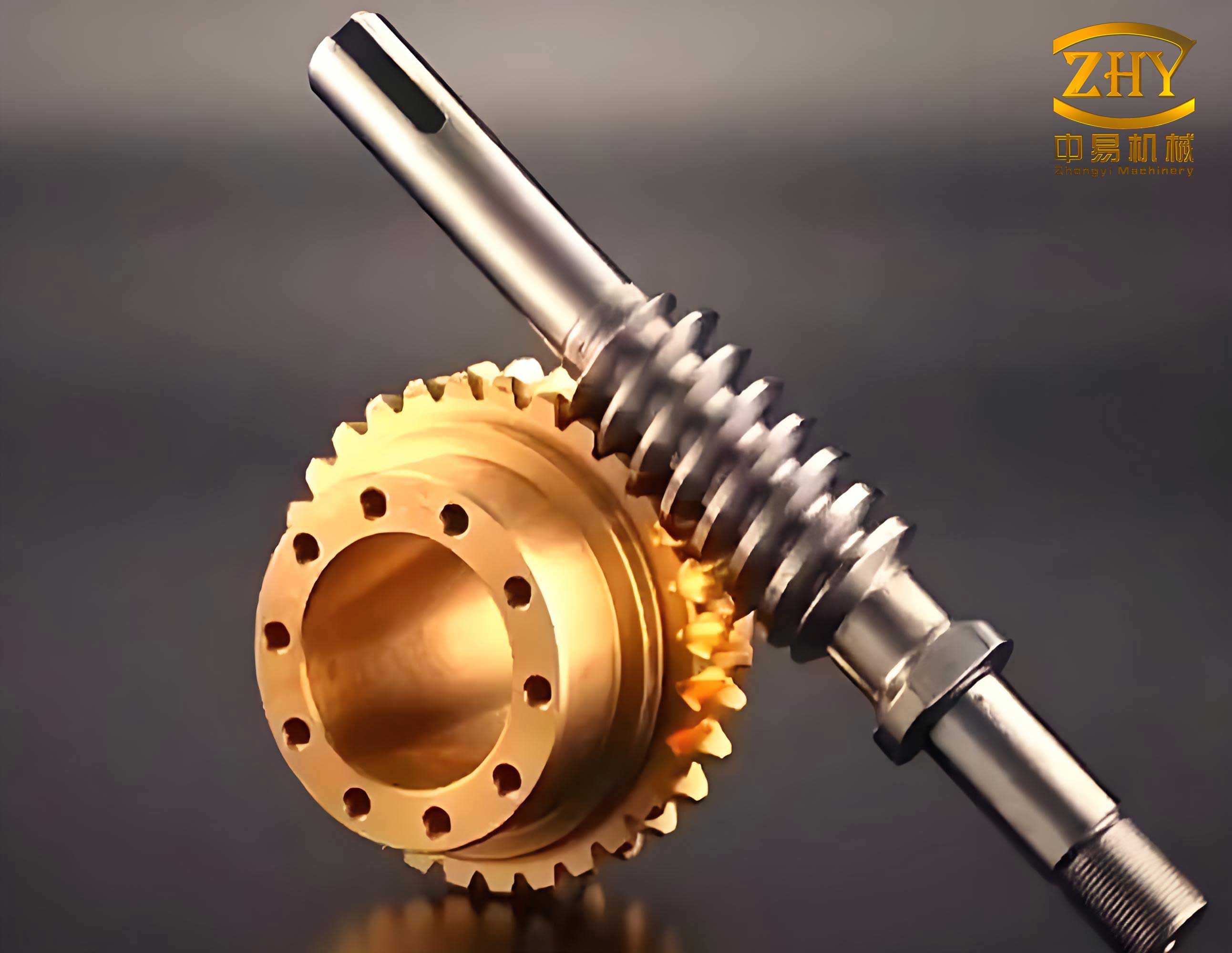
The primary objective is to minimize the volume of the bronze ring in the screw gear’s worm wheel. The volume \( V \) of this annular ring, as illustrated in the accompanying figure, is a function of its key dimensions: the outer diameter \( d_e \), the inner diameter \( d_0 \), and the face width \( b \). The fundamental geometric relationship is given by:
$$ V = \frac{\pi b (d_e^2 – d_0^2)}{4} $$
These dimensions are not independent but are intrinsically linked to the basic design parameters of the screw gear drive. The worm wheel’s outer diameter \( d_e \) is related to its addendum diameter \( d_{a2} \) and the module \( m \), while the inner diameter \( d_0 \) is related to its root diameter \( d_{f2} \). The face width \( b \) is typically proportional to the worm’s addendum diameter. By expressing all these dimensions in terms of the fundamental screw gear parameters, we can construct the objective function.
For a screw gear set, the worm wheel’s number of teeth \( z_2 \) is determined by the gear ratio \( u \) and the worm’s number of starts (threads) \( z_1 \), i.e., \( z_2 = u z_1 \). The worm wheel addendum and root diameters are \( d_{a2} = m(z_2 + 2) \) and \( d_{f2} = m(z_2 – 2.4) \), respectively, where \( m \) is the module. Common design practice often sets the ring’s outer diameter as \( d_e = d_{a2} + 6m/(z_1+2) \) and the inner diameter as \( d_0 = d_{f2} – 2m \). The face width is commonly taken as \( b = \xi d_{a1} \), where \( d_{a1} = m(q+2) \) is the worm’s addendum diameter, \( q \) is the diameter factor (defining the worm’s pitch diameter as \( d_1 = mq \)), and \( \xi \) is a face width coefficient (often 0.75 for \( z_1=1,2 \) and 0.67 for \( z_1=3,4 \)).
Substituting these relationships, the volume of the screw gear’s bronze ring becomes:
$$ V = \frac{\pi \xi m (q+2)}{4} \left[ \left( m(z_2+2) + \frac{6m}{z_1+2} \right)^2 – \left( m(z_2 – 4.4) \right)^2 \right] $$
Replacing \( z_2 \) with \( u z_1 \) and simplifying, we arrive at the objective function in terms of the core design variables:
$$ V = f(z_1, m, q) = \frac{\pi \xi m^3 (q+2)}{4} \left[ \left( u z_1 + 2 + \frac{6}{z_1+2} \right)^2 – (u z_1 – 4.4)^2 \right] $$
Since the gear ratio \( u \) is usually specified by the application requirements, and \( \xi \) is determined by \( z_1 \), the independent design variables are naturally selected as the worm number of starts \( z_1 \), the module \( m \), and the diameter factor \( q \). We define the design vector as:
$$ \mathbf{X} = [x_1, x_2, x_3]^T = [z_1, m, q]^T $$
Thus, the formal optimization problem is to minimize \( f(\mathbf{X}) \).
| Variable | Symbol | Design Vector Component | Role |
|---|---|---|---|
| Worm Number of Starts | \( z_1 \) | \( x_1 \) | Affects efficiency, lead angle, and wheel size. |
| Module | \( m \) | \( x_2 \) | Governs tooth size and overall gear dimensions. |
| Diameter Factor | \( q \) | \( x_3 \) | Controls worm stiffness and contact conditions. |
The minimization of the screw gear bronze volume is not unconstrained. The design must satisfy a set of boundary conditions dictated by standard practice and performance requirements dictated by strength and rigidity. These constraints ensure the resulting screw gear drive is functional, reliable, and manufacturable.
Boundary Constraints: These arise from recommended ranges for the design variables based on empirical knowledge and manufacturing standards.
- Worm Starts: For power transmission, the worm typically has \( z_1 = 2 \) to \( 4 \).
$$ g_1(\mathbf{X}) = 4 – x_1 \ge 0, \quad g_2(\mathbf{X}) = x_1 – 2 \ge 0 $$ - Worm Wheel Teeth: To avoid undercutting and ensure smooth operation, \( z_2 = u x_1 \) should be between 30 and 80.
$$ g_3(\mathbf{X}) = 80 – u x_1 \ge 0, \quad g_4(\mathbf{X}) = u x_1 – 30 \ge 0 $$ - Module: Standard modules for power screw gears usually fall within a specific range, e.g., 2 mm to 18 mm.
$$ g_5(\mathbf{X}) = 18 – x_2 \ge 0, \quad g_6(\mathbf{X}) = x_2 – 2 \ge 0 $$ - Diameter Factor: Corresponding to the module range, \( q \) is typically between 8 and 16 to ensure a sufficiently rigid worm.
$$ g_7(\mathbf{X}) = 16 – x_3 \ge 0, \quad g_8(\mathbf{X}) = x_3 – 8 \ge 0 $$
Performance Constraints: These are derived from the mechanical integrity requirements of the screw gear drive.
- Surface Contact Strength: The primary failure mode for screw gears is surface pitting on the worm wheel teeth. The contact stress must not exceed the allowable stress \( [\sigma_H] \) of the bronze material. The condition derived from the Hertzian contact theory is:
$$ m^3 q \ge K T_2 \left( \frac{500}{z_2 [\sigma_H]} \right)^2 $$
where \( K \) is the load factor and \( T_2 \) is the output torque on the worm wheel. This yields the inequality constraint:
$$ g_9(\mathbf{X}) = x_2^3 x_3 – K T_2 \left( \frac{500}{u x_1 [\sigma_H]} \right)^2 \ge 0 $$ - Worm Shaft Deflection: Excessive bending of the worm shaft can lead to poor tooth contact and localized overload. The maximum deflection \( y \) at the worm’s mid-span should be less than \( m/50 \) for proper meshing. The deflection formula, considering the worm as a simply supported beam under combined tangential \( F_{t1} \) and radial \( F_{r1} \) forces, is:
$$ y = \frac{\sqrt{F_{t1}^2 + F_{r1}^2} \cdot L^3}{48 E J} \le \frac{m}{50} $$
Here, \( L \approx 0.9 d_2 = 0.9 m u z_1 \) is the support span, \( J = \pi d_{f1}^4 / 64 = \pi m^4 (q – 2.4)^4 / 64 \) is the area moment of inertia of the worm’s root diameter, \( E \) is the modulus of elasticity, \( F_{t1} = 2T_1/(m q) = 2T_2/(u m q) \), and \( F_{r1} \approx F_{t2} \tan \alpha = (2T_2 / d_2) \tan 20^\circ \). Substituting and rearranging gives the stiffness constraint:
$$ g_{10}(\mathbf{X}) = C x_2^5 (x_3 – 2.4)^4 – T_2 \sqrt{ \left( \frac{x_1}{x_3} \right)^2 + \tan^2 20^\circ } \ge 0 $$
where \( C \) is a constant consolidating \( \pi, E, 0.9^3 \), etc.
| Constraint | Type | Mathematical Form \( g_i(\mathbf{X}) \ge 0 \) | Physical Basis |
|---|---|---|---|
| \( g_1, g_2 \) | Boundary | \( 4 – x_1 \), \( x_1 – 2 \) | Worm start number range. |
| \( g_3, g_4 \) | Boundary | \( 80 – u x_1 \), \( u x_1 – 30 \) | Worm wheel tooth count range. |
| \( g_5, g_6 \) | Boundary | \( 18 – x_2 \), \( x_2 – 2 \) | Standard module range. |
| \( g_7, g_8 \) | Boundary | \( 16 – x_3 \), \( x_3 – 8 \) | Diameter factor range. |
| \( g_9 \) | Performance | \( x_2^3 x_3 – K T_2 \left( \frac{500}{u x_1 [\sigma_H]} \right)^2 \) | Surface contact strength (pitting resistance). |
| \( g_{10} \) | Performance | \( C x_2^5 (x_3-2.4)^4 – T_2 \sqrt{ (x_1/x_3)^2 + \tan^2 20^\circ } \) | Worm shaft stiffness (deflection limit). |
The formulated problem is a nonlinear constrained optimization with three variables and ten constraints. A powerful and classical method for solving such problems is the Exterior Penalty Function Method. This method transforms the constrained problem into a sequence of unconstrained problems. A penalty term is added to the original objective function \( f(\mathbf{X}) \); this term increases sharply when constraints are violated. The composite function, for the \( k \)-th iteration, is:
$$ \Phi(\mathbf{X}, r^{(k)}) = f(\mathbf{X}) + r^{(k)} \sum_{i=1}^{10} \left[ \min(0, g_i(\mathbf{X})) \right]^2 $$
Here, \( r^{(k)} \) is a positive penalty parameter that increases (\( r^{(k+1)} = c \cdot r^{(k)}, c > 1 \)) as the iterations progress, forcing the solution to adhere to the feasible region. The unconstrained minimization of \( \Phi(\mathbf{X}, r^{(k)}) \) for increasingly larger \( r^{(k)} \) converges to the solution of the original constrained problem. Algorithms like the Davidon-Fletcher-Powell (DFP) or Broyden–Fletcher–Goldfarb–Shanno (BFGS) method can be used for each unconstrained minimization.
To demonstrate the practical application and benefits of this optimization framework for screw gear design, consider a concrete example with the following given parameters:
| Parameter | Symbol | Value | Unit |
|---|---|---|---|
| Output Torque | \( T_2 \) | 546,550 | N·mm |
| Gear Ratio | \( u \) | 26.39 | – |
| Load Factor | \( K \) | 1.1 | – |
| Allowable Contact Stress | \( [\sigma_H] \) | 180 | MPa |
| Face Width Coefficient | \( \xi \) | 0.67 (for \( z_1 \approx 3 \)) | – |
The complete optimization model becomes:
$$ \text{Minimize: } f(\mathbf{X}) = \frac{\pi \cdot 0.67 \cdot x_2^3 (x_3+2)}{4} \left[ \left( 26.39x_1 + 2 + \frac{6}{x_1+2} \right)^2 – (26.39x_1 – 4.4)^2 \right] $$
subject to the constraints \( g_1(\mathbf{X}) \) through \( g_{10}(\mathbf{X}) \) with numerical values inserted. For instance:
$$ g_9(\mathbf{X}) = x_2^3 x_3 – 1.1 \cdot 546550 \cdot \left( \frac{500}{26.39 x_1 \cdot 180} \right)^2 \ge 0 $$
$$ g_{10}(\mathbf{X}) = 5498 \cdot x_2^5 (x_3 – 2.4)^4 – 546550 \cdot \sqrt{ \left( \frac{x_1}{x_3} \right)^2 + 0.1325 } \ge 0 $$
The constant in \( g_{10} \) (5498) incorporates \( E \), \( \pi \), and other geometric factors from the detailed derivation.
Applying the exterior penalty function method, the algorithm converges to an optimal solution. The raw optimization results and a practical rounded-off design are presented below, alongside a conventional design obtained by standard handbook procedures for comparison.
| Design Parameter | Raw Optimal Result | Rounded Practical Design | Conventional Design |
|---|---|---|---|
| Worm Starts (\( z_1 \)) | 3.0315 | 3 | 2 |
| Module (\( m \)) [mm] | 3.5648 | 4 | 6.3 |
| Diameter Factor (\( q \)) | 16.0000 | 16 | 7.936 |
| Bronze Ring Volume (\( V \)) [mm³] | 7.2238 × 10⁵ | 1.0106 × 10⁶ | 1.2100 × 10⁶ |
The results are highly insightful. The optimization algorithm naturally pushes the screw gear design towards a configuration that minimizes material volume. It selects a higher number of worm starts (\( z_1 \approx 3 \)) compared to the conventional design (\( z_1=2 \)). This increases the lead angle, which generally improves efficiency and allows for a smaller worm wheel for the same ratio, directly contributing to volume reduction. More significantly, the optimal module is drastically smaller (3.56 mm vs. 6.3 mm). Since volume scales with \( m^3 \), reducing the module has the most profound effect on saving material. To compensate for the reduced size and maintain strength (contact and stiffness), the algorithm maximizes the diameter factor \( q \) to its upper bound (16), which increases the worm’s pitch diameter and cross-sectional area, thereby enhancing its stiffness and improving the contact pattern on the smaller worm wheel teeth.
The raw optimal volume is approximately 722,380 mm³. After rounding the variables to standard/preferred values (z₁=3, m=4, q=16), the volume increases to about 1,010,600 mm³. Crucially, even this rounded optimal design uses **16.5% less bronze** than the conventional design (1,210,000 mm³). This demonstrates the substantial economic benefit of applying formal optimization to screw gear design.
The optimization of the screw gear drive reveals intricate interactions between the design variables. The choice of the worm’s number of starts \( z_1 \) is pivotal. While a single-start worm offers the highest theoretical reduction per size, it often results in a lower lead angle, potentially poorer efficiency, and crucially for this problem, a larger worm wheel diameter for a given ratio and center distance. The optimization model correctly identifies that a moderate increase to \( z_1 = 3 \) allows a more compact wheel. The module \( m \) is the dominant factor in the objective function. The algorithm’s drive to minimize \( m \) is strongly checked by the contact stress constraint \( g_9 \) and the stiffness constraint \( g_{10} \). The contact stress constraint is approximately of the form \( m^3 q \propto 1/z_1^2 \), indicating that a smaller \( m \) can be tolerated if \( q \) is increased or \( z_1 \) is increased. The stiffness constraint \( g_{10} \), which depends on \( m^5 q^4 \), is even more severe and effectively prevents the module from becoming too small unless the diameter factor \( q \) is sufficiently large. This explains why the optimal solution pushes \( q \) to its maximum allowable value. The constraints \( g_9 \) and \( g_{10} \) are typically active at the optimum, meaning they are satisfied as equalities, which is characteristic of a well-formulated optimization where the design is limited by performance limits, not just arbitrary boundaries.
The successful implementation of this screw gear optimization model highlights several important considerations for the design engineer. First, the accuracy of the model depends heavily on the correct specification of input parameters, especially the load factor \( K \) and the allowable contact stress \( [\sigma_H] \), which may themselves depend on material, lubrication, and lifecycle requirements. Second, while the objective here was volume minimization, the model could be adapted for other goals, such as maximizing efficiency, minimizing center distance, or even a multi-objective formulation. Third, the rounded solution, while slightly less optimal than the raw mathematical result, proves that the method yields practical, implementable designs with clear advantages over traditional approaches. The systematic nature of this optimization process for screw gears ensures that no potential for material and cost savings is overlooked, promoting sustainable engineering practices.
| Design Variable | Trend in Optimal Solution | Primary Governing Constraint(s) | Effect on Bronze Volume |
|---|---|---|---|
| Worm Starts (\( z_1 \)) | Increased from conventional value. | Lower bound \( g_2 \), Contact \( g_9 \). | Reduces wheel diameter, decreasing volume. |
| Module (\( m \)) | Significantly decreased. | Contact \( g_9 \) and Stiffness \( g_{10} \). | Cubic reduction in volume; most critical variable. |
| Diameter Factor (\( q \)) | Increased to upper bound. | Upper bound \( g_7 \), Stiffness \( g_{10} \). | Enables use of smaller module by improving stiffness. |
In conclusion, the systematic optimization of screw gear design, with the explicit objective of minimizing the volume of expensive alloy in the worm wheel ring, presents a powerful methodology for achieving significant cost reduction and material efficiency. By establishing a mathematical model with three key design variables—worm starts, module, and diameter factor—and subjecting them to a comprehensive set of ten geometric and mechanical constraints, an optimal design space is rigorously defined. The application of nonlinear programming techniques, such as the exterior penalty function method, allows for the efficient navigation of this space to find the best possible combination of parameters. The provided case study unequivocally demonstrates the value of this approach, yielding a design that uses over 16% less material than a conventionally designed screw gear while meeting all performance criteria. This framework not only provides immediate economic benefits but also serves as a template for optimizing other aspects of screw gear performance, solidifying the role of computational optimization in advanced mechanical design.