
In mechanical engineering, screw gear transmissions, commonly referred to as worm drives, play a pivotal role in transmitting motion and power between non-intersecting shafts, typically at right angles. These systems are prized for their high reduction ratios, compact design, smooth operation, and quiet performance, making them indispensable in industries such as mining, metallurgy, transportation, and lifting machinery. However, traditional design methods for screw gear transmissions often rely on empirical knowledge and iterative trial-and-error approaches, which are time-consuming, labor-intensive, and may not yield optimal solutions. This leads to drawbacks like high material costs and low transmission efficiency. To address these challenges, I propose a multi-objective fuzzy optimization design framework leveraging Matlab, which integrates fuzzy set theory to handle uncertainties in design constraints and aims to minimize volume and maximize efficiency. This approach not only streamlines the design process but also achieves superior performance, offering significant value for industrial applications.
The core of this methodology lies in constructing a fuzzy optimization mathematical model that accounts for the inherent vagueness in engineering specifications. By defining design variables, objective functions, and constraints with fuzzy boundaries, we can better reflect real-world scenarios where tolerances and performance criteria are not strictly binary. Through Matlab programming and its Optimization Toolbox, we solve the model efficiently, resulting in a design that significantly reduces the volume of the worm wheel rim and enhances transmission efficiency. This article delves into the detailed formulation of the model, the implementation in Matlab, and the outcomes, with an emphasis on practical insights. Throughout, I will refer to the system as a screw gear to underscore the gear-like interaction in worm drives, and I will incorporate multiple tables and equations to elucidate key concepts.
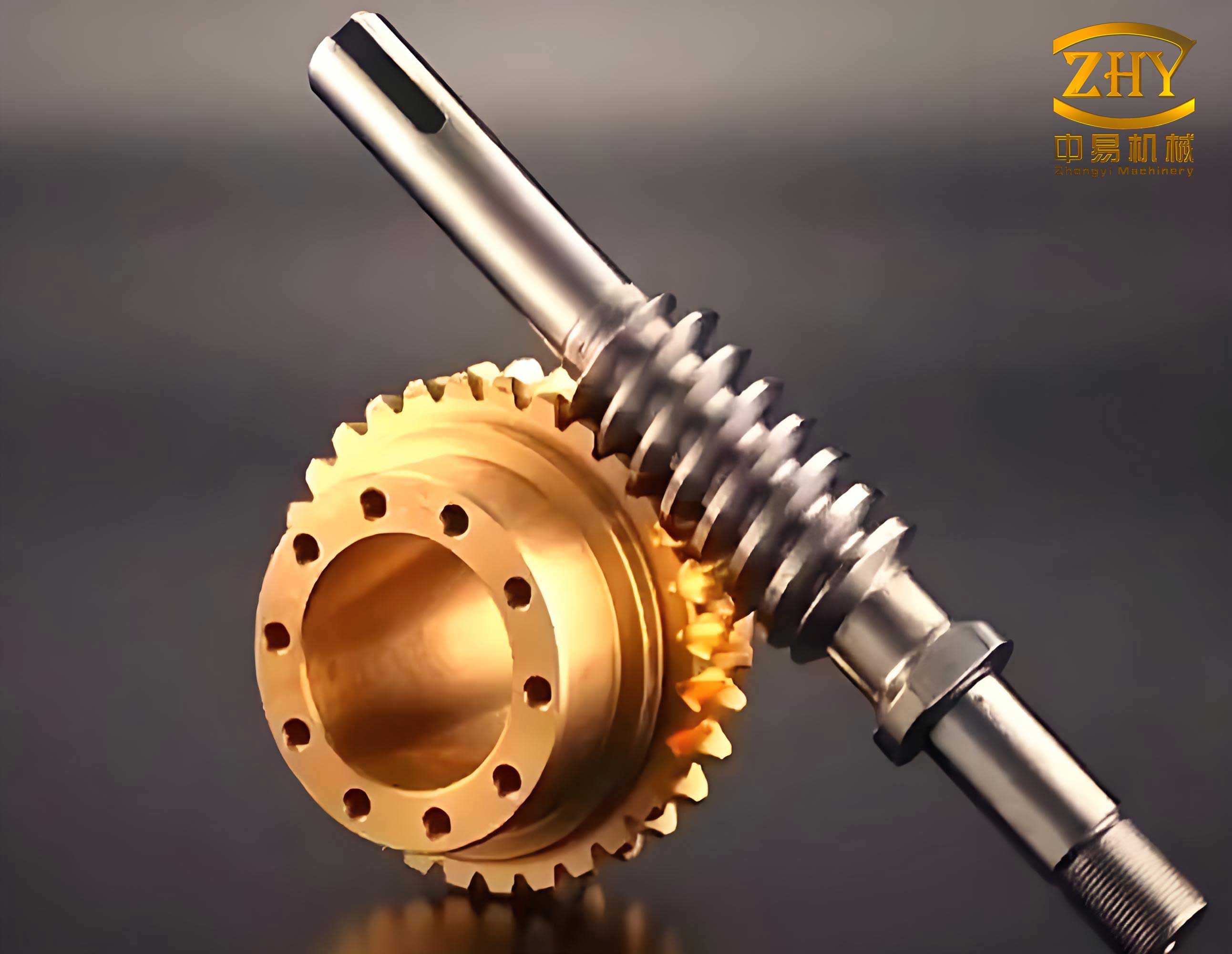
To begin, let’s establish the fuzzy optimization mathematical model. In any optimization problem, defining the design variables is crucial. For screw gear transmissions, I select three independent parameters that profoundly influence the objectives: the number of worm threads (denoted as $z_1$), the module ($m$), and the diameter factor ($q$). Thus, the design vector is expressed as:
$$\mathbf{X} = [x_1, x_2, x_3]^T = [z_1, m, q]^T.$$
These variables are chosen because they directly affect the gear geometry, load capacity, and efficiency, providing a balanced control over the design space.
Next, I formulate the objective functions. The primary goals are to minimize the volume of the worm wheel rim—which reduces material cost and weight—and to maximize the transmission efficiency. For the first objective, the volume of the rim portion, made of cast tin bronze, is considered. The volume $V$ is given by:
$$V = \frac{\pi}{4} (d_e^2 – d_0^2) B,$$
where $d_e$ is the maximum diameter of the rim, $d_0$ is the minimum diameter, and $B$ is the width. Using standard gear relations:
$$d_e = m(i z_1 + 3), \quad d_0 = m(i z_1 – 6.4), \quad B = 0.67 m(q + 2),$$
with $i = 20$ as the transmission ratio. Substituting these, the first objective function becomes:
$$f_1(\mathbf{X}) = 0.5262 m^3 (q + 2) [(i z_1 + 3)^2 – (i z_1 – 6.4)^2].$$
Simplifying with $i = 20$:
$$f_1(\mathbf{X}) = 0.5262 x_2^3 (x_3 + 2) [(20 x_1 + 3)^2 – (20 x_1 – 6.4)^2].$$
This function aims to minimize the volume, directly impacting cost savings in screw gear production.
For the second objective, maximizing transmission efficiency $\eta$, I instead minimize its reciprocal to align with minimization problems. The efficiency of a screw gear drive is:
$$\eta = 0.96 \frac{\tan \lambda}{\tan(\lambda + \rho_v)},$$
where $\lambda$ is the lead angle, $\tan \lambda = z_1 / q$, and $\rho_v$ is the equivalent friction angle, with $\tan \rho_v = f_v$. The equivalent friction coefficient $f_v$ depends on the sliding velocity $v_s$. Using empirical data fitted via Matlab curve fitting, $f_v$ is approximated as:
$$f_v = 0.0175192 e^{1.0460682 / v_s},$$
with sliding velocity:
$$v_s = \frac{m n_1}{19100} \sqrt{z_1^2 + q^2},$$
where $n_1 = 960$ rpm is the worm speed. Thus, the second objective function is:
$$f_2(\mathbf{X}) = \frac{1}{\eta} = \frac{\tan(\lambda + \rho_v)}{0.96 \tan \lambda} = \frac{z_1 q + f_v q^2}{0.96 z_1 q – 0.96 z_1^2 f_v} = \frac{x_1 x_3 + f_v x_3^2}{0.96 x_1 x_3 – 0.96 x_1^2 f_v}.$$
Minimizing $f_2(\mathbf{X})$ enhances the screw gear’s energy efficiency, a critical factor in sustainable design.
To combine these into a unified target, I employ a weighted sum method. Assigning weights $\omega_1 = 0.8$ for volume and $\omega_2 = 0.2$ for efficiency, and scaling $f_2(\mathbf{X})$ by $10^6$ to match the magnitude of $f_1(\mathbf{X})$, the unified objective function is:
$$f(\mathbf{X}) = 0.8 f_1(\mathbf{X}) + 0.2 \times 10^6 f_2(\mathbf{X}) = 0.420976 x_2^3 (x_3 + 2) [(20 x_1 + 3)^2 – (20 x_1 – 6.4)^2] – \frac{4.8 \times 10^6 (x_1 x_3 + f_v x_3^2)}{x_1 (x_3 – x_1 f_v)}.$$
This formulation balances the trade-offs between material usage and performance in screw gear systems.
Now, let’s address the constraints. In fuzzy optimization, constraints are not rigid but have transitional zones, reflecting real-world tolerances. I categorize constraints into boundary and performance types. For boundary constraints, based on screw gear design handbooks, I define fuzzy limits for each variable:
| Variable | Description | Fuzzy Lower Bound | Fuzzy Upper Bound | Standard Range |
|---|---|---|---|---|
| $z_1$ | Number of worm threads | 2 | 6 | 2–6 for power transmission |
| $m$ (mm) | Module | 2 | 18 | 2–18 for power transmission |
| $q$ | Diameter factor | 8 | 15 | 8–15 for efficiency |
| $z_2$ | Number of worm wheel teeth | 30 | 80 | 30–80 to avoid undercutting |
These bounds are fuzzified using membership functions, as detailed later. For performance constraints, which ensure the screw gear’s operational reliability, I consider five key aspects: contact stress, bending stress, shaft deflection, sliding velocity, and thermal balance. Each constraint is derived from mechanical principles and expressed as inequalities.
First, the contact fatigue strength constraint prevents surface pitting. The contact stress $\sigma_H$ must not exceed the allowable value $[\sigma_H]$. The formula is:
$$\sigma_H = Z_E \sqrt{\frac{9400 T_2 K_A K_V K_\beta}{d_1 d_2^2}} \leq [\sigma_H],$$
where $Z_E = 155 \sqrt{\text{MPa}}$ for steel worm and bronze wheel, $T_2 = 1268.36 \text{ N·m}$ is the output torque, $K_A = 1.0$, $K_V = 1.1$, $K_\beta = 1.0$ are factors, $d_1 = m q$ is the worm pitch diameter, and $d_2 = m i z_1$ is the wheel pitch diameter. Substituting values:
$$g_5(\mathbf{X}) = \frac{28066.176}{\sqrt{x_1^2 x_2^3 x_3}} \leq [\sigma_H].$$
The allowable $[\sigma_H]$ is fuzzy, with a transition range.
Second, the bending fatigue strength constraint avoids tooth breakage. The bending stress $\sigma_F$ is:
$$\sigma_F = \frac{666 T_2 K_A K_V K_\beta}{d_1 d_2 m} Y_{Fs} Y_\beta \leq [\sigma_F],$$
where $Y_{Fs}$ is the composite tooth form factor, approximated via curve fitting as $Y_{Fs} = 2.58 e^{-0.049 z_1}$, and $Y_\beta = 1 – \lambda/120^\circ$ is the lead angle factor. Thus:
$$g_6(\mathbf{X}) = \frac{119866.869}{x_1 x_2^3 x_3} e^{-0.049 x_1} \left(1 – \frac{\arctan(x_1/x_3)}{120}\right) \leq [\sigma_F].$$
Third, the shaft stiffness constraint limits worm deflection to prevent misalignment. The deflection $f$ at the meshing point is:
$$f = \frac{\sqrt{F_{r1}^2 + F_{t1}^2}}{48 E I} L^3 \leq [f],$$
where $F_{t1} = 2T_2/(i \eta m q)$, $F_{r1} = 2T_2 \tan \alpha/(m i z_1)$ with $\alpha = 20^\circ$, $E = 2.1 \times 10^5 \text{ MPa}$, $I = \pi m^4 (q – 2.4)^4/64$, and $L = 1.1 m(i z_1 + 2)$. Simplifying:
$$g_7(\mathbf{X}) = \frac{3.411852 \times 10^{-4} (20 x_1 + 2)^3 \sqrt{(0.36397/x_1)^2 + (1.17647/x_3)^2}}{(x_3 – 2.4)^4 x_2^2} \leq [f].$$
Fourth, the sliding velocity constraint mitigates wear and overheating:
$$g_8(\mathbf{X}) = 0.05026178 x_2 \sqrt{x_1^2 + x_3^2} \leq [v_s].$$
Fifth, the thermal balance constraint ensures heat dissipation:
$$\Delta t = \frac{1000 P (1 – \eta)}{k_s A} \leq [\Delta t],$$
where $P = 7.5 \text{ kW}$ is input power, $k_s = 15 \text{ W/(m}^2\cdot^\circ\text{C)}$, and $A = 0.33 (a/100)^{1.75}$ with $a = m(q + i z_1)/2$ as center distance. This yields:
$$g_9(\mathbf{X}) = \frac{2417407.226}{[x_2 (x_3 + 20 x_1)]^{1.75}} \leq [\Delta t].$$
All performance constraints have fuzzy allowable values, which I model using linear membership functions. The membership function $\mu_{g_j}(\mathbf{X})$ for a constraint $g_j(\mathbf{X})$ is defined as:
$$\mu_{g_j}(\mathbf{X}) =
\begin{cases}
1 & \text{if } g_j(\mathbf{X}) \leq \sigma_j^l, \\
\frac{\sigma_j^u – g_j(\mathbf{X})}{\sigma_j^u – \sigma_j^l} & \text{if } \sigma_j^l \leq g_j(\mathbf{X}) \leq \sigma_j^u, \\
0 & \text{if } g_j(\mathbf{X}) \geq \sigma_j^u,
\end{cases}$$
where $\sigma_j^l$ and $\sigma_j^u$ are the lower and upper bounds of the fuzzy allowable interval. Similarly, for boundary constraints, the membership function $\mu_{x_j}$ is piecewise linear. To determine these intervals, I use the expansion coefficient method, with coefficients $\beta^+ = 1.05$ for upper bounds and $\beta^- = 0.85$ for lower bounds, applied to conventional design values. The resulting fuzzy allowable intervals are summarized in the table below.
| Constraint | Symbol | Conventional Value | Fuzzy Lower Bound ($\sigma_j^l$) | Fuzzy Upper Bound ($\sigma_j^u$) |
|---|---|---|---|---|
| Contact stress (MPa) | $[\sigma_H]$ | 166.57 | 141.58 | 174.90 |
| Bending stress (MPa) | $[\sigma_F]$ | 38.16 | 32.44 | 40.07 |
| Deflection (mm) | $[f]$ | $m/50$ | $0.017m$ | $0.021m$ |
| Sliding velocity (m/s) | $[v_s]$ | 16 | 13.6 | 16.8 |
| Temperature rise (°C) | $[\Delta t]$ | 60 | 51 | 63 |
| Worm threads | $z_1$ | 2–6 | 1.7–6.3 | 2–6.3 |
| Module (mm) | $m$ | 2–18 | 1.7–18.9 | 2–18.9 |
| Diameter factor | $q$ | 8–15 | 6.8–15.75 | 8–15.75 |
| Wheel teeth | $z_2$ | 30–80 | 25.5–84 | 30–84 |
To convert the fuzzy optimization problem into a crisp one, I determine the optimal level-cut $\lambda^*$ using fuzzy comprehensive evaluation. Considering factors like design safety, cost, and manufacturability, and applying the M(•,+) operator, I obtain $\lambda^* = 0.6$. This means we consider all constraints with membership values at least 0.6 as acceptable. Thus, the non-fuzzy optimization model is formulated by tightening the bounds: for each constraint $g_j(\mathbf{X})$, the allowable value becomes $\sigma_j^l + \lambda^* (\sigma_j^u – \sigma_j^l)$. For example, for contact stress, the crisp bound is $141.58 + 0.6(174.90 – 141.58) = 141.58 + 19.99 = 161.57 \text{ MPa}$. Similarly, for variables, the bounds are adjusted. The full set of crisp constraints is:
- $1.88 \leq x_1 \leq 6.12$
- $28.2 \leq 20 x_1 \leq 81.6$
- $1.88 \leq x_2 \leq 18.36$
- $7.52 \leq x_3 \leq 15.35$
- $g_5(\mathbf{X}) \leq 169.92 \text{ MPa}$
- $g_6(\mathbf{X}) \leq 38.924 \text{ MPa}$
- $g_7(\mathbf{X}) \leq 0.0204 x_2 \text{ mm}$
- $g_8(\mathbf{X}) \leq 16.32 \text{ m/s}$
- $g_9(\mathbf{X}) \leq 61.2 ^\circ\text{C}$
With the model established, I implement the optimization in Matlab. The process involves writing M-files for the objective function and nonlinear constraints, then using the fmincon solver from the Optimization Toolbox. The objective function is coded in a file named myobj.m:
function f = myobj(x)
fv = 0.0175192 * exp(1.0460682 / (0.05026178 * x(2) * sqrt(x(1)^2 + x(3)^2)));
f = 0.420976 * x(2)^3 * (x(3) + 2) * ((20*x(1) + 3)^2 - (20*x(1) - 6.4)^2) ...
    - (4.8e6 * (x(1)*x(3) + fv*x(3)^2)) / (x(1) * (x(3) - x(1)*fv));
end
The nonlinear constraints are in mycon.m:
function [c, ceq] = mycon(x)
fv = 0.0175192 * exp(1.0460682 / (0.05026178 * x(2) * sqrt(x(1)^2 + x(3)^2)));
c(1) = 28066.176 / sqrt(x(1)^2 * x(2)^3 * x(3)) - 169.92;
c(2) = 119866.869 * exp(-0.049*x(1)) * (1 - atan(x(1)/x(3))/120) / (x(1)*x(2)^3*x(3)) - 38.924;
c(3) = 3.411852e-4 * (20*x(1) + 2)^3 * sqrt((0.36397/x(1))^2 + (1.17647/x(3))^2) / ((x(3)-2.4)^4 * x(2)^2) - 0.0204*x(2);
c(4) = 0.05026178 * x(2) * sqrt(x(1)^2 + x(3)^2) - 16.32;
c(5) = 2417407.226 / (x(2) * (x(3) + 20*x(1)))^1.75 - 61.2;
ceq = [];
end
Then, in the main script, I set bounds, linear constraints, and initial guesses:
lb = [1.7, 1.7, 6.8];
ub = [6.3, 18.9, 15.75];
x0 = [1.7, 1.7, 6.8];
A = [-1 0 0; 1 0 0; 0 -1 0; 0 1 0; 0 0 -1; 0 0 1];
b = [-1.88; 6.12; -1.88; 18.36; -7.52; 15.35];
options = optimset('Display', 'off', 'LargeScale', 'off');
[x_opt, fval] = fmincon(@myobj, x0, A, b, [], [], lb, ub, @mycon, options);
Running this yields the optimal solution: $\mathbf{X}^* = [4.08, 4.743, 15.35]$. For practical screw gear design, these are rounded to standard values: $z_1 = 4$, $m = 5 \text{ mm}$, $q = 15$. Comparing with a traditional design ($z_1 = 2$, $m = 8 \text{ mm}$, $q = 10$), the improvements are substantial. The volume of the worm wheel rim decreases from $2.327958 \times 10^6 \text{ mm}^3$ to $1.64606 \times 10^6 \text{ mm}^3$, a reduction of 29.3%. The transmission efficiency increases from 0.8586 to 0.8787, a gain of 2.34%. These results demonstrate the efficacy of the fuzzy optimization approach in enhancing screw gear performance.
To further illustrate the benefits, let’s analyze the sensitivity of the objectives to design variables. Using Matlab’s parametric tools, I vary each variable within its range while holding others constant at optimal values, and compute the objective functions. The trends show that $z_1$ has a strong influence on efficiency, while $m$ dominates volume. This underscores the importance of multi-objective optimization in screw gear design, as single-factor adjustments may lead to suboptimal trade-offs.
| Variable | Range | Effect on Volume ($f_1$) | Effect on Efficiency ($f_2$) | Recommendation |
|---|---|---|---|---|
| $z_1$ | 2–6 | Decreases with higher $z_1$ | Improves significantly with higher $z_1$ | Prefer higher $z_1$ for efficiency |
| $m$ (mm) | 2–18 | Increases cubically with $m$ | Minor improvement with moderate $m$ | Keep $m$ low to reduce volume |
| $q$ | 8–15 | Increases linearly with $q$ | Improves with higher $q$ up to a point | Optimize $q$ for balance |
Moreover, the fuzzy constraints provide robustness against uncertainties. For instance, in real-world screw gear applications, operating conditions like load fluctuations or temperature variations can be accommodated by the fuzzy allowable intervals. This flexibility is a key advantage over deterministic methods, which might fail under off-design conditions.
In conclusion, the multi-objective fuzzy optimization design for screw gear transmissions, implemented via Matlab, offers a systematic and efficient approach to overcoming the limitations of traditional design. By integrating fuzzy set theory, we handle the vagueness in engineering constraints, leading to a more realistic model. The optimization results confirm significant reductions in material volume and enhancements in efficiency, directly addressing cost and performance issues. This methodology not only streamlines the design process but also provides a framework for adapting to various screw gear configurations, such as those in automotive or industrial machinery. Future work could extend this to other gear types or incorporate dynamic factors, but the current approach already marks a substantial step forward in mechanical design optimization.
Throughout this discussion, I have emphasized the term “screw gear” to highlight the gear-like nature of worm drives, and I have used numerous equations and tables to clarify the technical details. The integration of Matlab tools makes this approach accessible to engineers, enabling rapid prototyping and optimization. As industries strive for greater sustainability and cost-effectiveness, such advanced design techniques will become increasingly vital, and screw gear systems will continue to evolve with these innovations.