
In modern manufacturing, gears serve as critical components for power transmission across various industries, including automotive, aerospace, and heavy machinery. Among the numerous gear production techniques, gear hobbing stands out due to its versatility, efficiency, and applicability for both roughing and semi-finishing operations. The emergence of high-speed dry gear hobbing has revolutionized this field by eliminating cutting fluids, thereby promoting environmentally friendly and cost-effective production. This shift aligns with the growing demand for sustainable manufacturing practices. However, the success of high-speed dry gear hobbing heavily relies on the optimal selection of process parameters, which directly influence performance metrics such as tool life, machining accuracy, energy consumption, and production costs. In this article, I will explore the recent advancements in process parameter optimization for high-speed dry gear hobbing, delving into the underlying principles, key variables, objective functions, constraints, simulation techniques, and optimization methodologies. By integrating tables and mathematical formulations, I aim to provide a comprehensive overview that underscores the importance of systematic parameter tuning in enhancing the efficiency and sustainability of gear hobbing operations.
The fundamental principle of gear hobbing involves a generating process where a hob—a cutting tool with multiple helical teeth—engages with a gear blank to form the desired tooth profile through simultaneous rotational and translational motions. This process relies on the kinematic relationship between the hob and the workpiece, ensuring precise tooth generation. In high-speed dry gear hobbing, the absence of cutting fluids necessitates higher cutting speeds to dissipate heat through chip removal, reducing thermal deformation and improving surface integrity. The basic motions include the primary rotation of the hob, the indexing motion of the gear blank to maintain proper meshing, and the axial feed motion of the hob along the gear axis. Understanding these motions is crucial for parameter optimization, as they define the interaction dynamics that affect cutting forces, temperature distribution, and tool wear. The complexity of gear hobbing arises from its intermittent cutting nature, where each hob tooth engages discontinuously, leading to varying load conditions. This necessitates a detailed analysis of the process variables to achieve optimal performance. For instance, the hob’s geometry, such as its diameter, number of starts, and helix angle, significantly impacts the chip formation and heat generation. Additionally, the machine tool’s characteristics, including spindle dynamics and thermal stability, play a vital role in maintaining accuracy under high-speed conditions. By examining these aspects, we can identify the key parameters that require optimization to balance competing objectives like productivity and tool longevity.
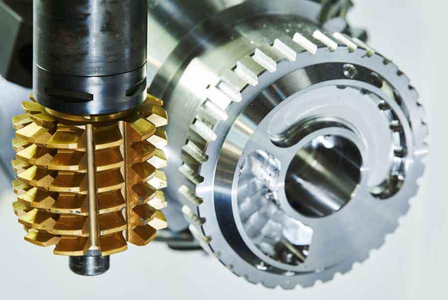
Optimization variables in high-speed dry gear hobbing encompass a broad range of factors that directly or indirectly influence the machining outcome. These variables can be categorized into material properties, tool parameters, machine settings, and cutting conditions. Each category interacts with the others, creating a multivariate optimization problem. For example, the workpiece material—such as 40Cr, 45 steel, or 20CrMnTi—affects machinability, which in turn dictates suitable cutting parameters. Similarly, the hob material, often comprising carbide, powder metallurgy high-speed steel (PM-HSS), or polycrystalline cubic boron nitride (PCBN), determines wear resistance and thermal stability. Tool geometry parameters, like hob diameter ($d_{a0}$), number of starts ($z_0$), and rake angles, influence chip flow and cutting forces. Machine-related variables include spindle speed capabilities, feed drive accuracy, and thermal compensation systems. Lastly, cutting parameters such as cutting speed ($v_c$), feed rate ($f$), and depth of cut ($a_p$) are primary decision variables that control the machining process. To illustrate the interdependence of these variables, Table 1 summarizes key optimization variables and their typical ranges in high-speed dry gear hobbing.
| Category | Variable | Description | Typical Range/Values |
|---|---|---|---|
| Workpiece Material | Material type | Steel alloys like 40Cr, 20CrMnTi | Various grades |
| Tool Material | Hob composition | Carbide, PM-HSS, PCBN | Depends on application |
| Tool Geometry | Hob diameter ($d_{a0}$) | Diameter of the hob | 50–200 mm |
| Tool Geometry | Number of starts ($z_0$) | Number of helical threads on hob | 1–4 |
| Machine Parameters | Spindle speed ($n$) | Rotational speed of hob | 1000–5000 rpm |
| Machine Parameters | Axial feed rate ($f_a$) | Feed along gear axis | 0.1–2 mm/rev |
| Cutting Parameters | Cutting speed ($v_c$) | Peripheral speed of hob | 100–300 m/min |
| Cutting Parameters | Feed per tooth ($f_z$) | Feed per hob tooth | 0.05–0.3 mm/tooth |
| Cutting Parameters | Depth of cut ($a_p$) | Radial engagement | 1–5 mm |
The selection of these variables is critical because they determine the economic and technical feasibility of the gear hobbing process. For instance, increasing the cutting speed in dry gear hobbing can enhance productivity but may accelerate tool wear due to elevated temperatures. Conversely, reducing the feed rate might improve surface finish but at the cost of longer machining times. Therefore, a systematic approach to parameter optimization is essential to navigate these trade-offs. Recent studies have focused on developing models that correlate these variables with performance metrics, enabling data-driven optimization. In the following sections, I will delve into the objective functions that quantify these performance metrics, providing a foundation for optimization models.
Objective functions in high-speed dry gear hobbing optimization typically aim to minimize or maximize certain criteria that reflect process efficiency, cost, quality, and sustainability. Common objectives include machining time, production cost, energy consumption, tool life, and gear accuracy. These objectives are often conflicting, necessitating multi-objective optimization approaches. For example, minimizing machining time usually requires higher cutting speeds and feeds, which can increase tool wear and energy usage. Thus, defining appropriate objective functions is a key step in the optimization process. The machining time ($t_m$) for a single gear in dry gear hobbing can be expressed as:
$$ t_m = \frac{\pi \cdot d_{a0} \cdot \left( a_p + \frac{1.25 \cdot m_n \cdot \sin \delta}{\tan \alpha} + B \right) + 4}{1000 \cdot f \cdot z_0 \cdot v_c} \cdot \frac{\pi \cdot d_{a0} \cdot z}{1} $$
where $m_n$ is the normal module, $\delta$ is the hob lead angle, $\alpha$ is the pressure angle, $B$ is the face width of the gear, and $z$ is the number of gear teeth. This equation highlights how parameters like hob diameter, feed rate, and cutting speed directly affect productivity. Another critical objective is production cost ($C$), which encompasses machine depreciation, tooling expenses, and overheads. A simplified cost model for dry gear hobbing can be written as:
$$ C = C_m \cdot t_m + \frac{C_{t0} + k \cdot (C_1 + C_2)}{(k+1) \cdot N} $$
Here, $C_m$ is the machine cost per unit time, $C_{t0}$ is the initial hob cost, $k$ is the number of regrinding and recoating cycles, $C_1$ and $C_2$ are costs per regrinding and recoating, respectively, and $N$ is the number of gears produced per hob life. Energy consumption ($E$) is another vital objective, especially for sustainable manufacturing. It can be modeled as the sum of fixed energy (e.g., machine idle) and variable energy (e.g., cutting power):
$$ E = P_{\text{idle}} \cdot t_{\text{idle}} + P_{\text{cut}} \cdot t_m $$
where $P_{\text{idle}}$ and $P_{\text{cut}}$ are power demands during idle and cutting, respectively. Tool life ($L$) is often predicted using empirical models like Taylor’s tool life equation, adapted for gear hobbing:
$$ v_c \cdot T^n = C $$
with $T$ being tool life in minutes, $n$ an exponent, and $C$ a constant. Gear accuracy objectives, such as minimizing tooth profile error ($\delta_y$) and tooth direction error ($\delta_x$), are also considered, typically through statistical or simulation-based models. These objective functions form the basis of optimization problems, where the goal is to find parameter sets that yield desirable values across multiple criteria. Table 2 summarizes common objective functions and their mathematical representations in high-speed dry gear hobbing optimization.
| Objective | Mathematical Formulation | Description |
|---|---|---|
| Machining Time | $t_m = f(d_{a0}, f, v_c, \text{geometry})$ | Time to complete one gear |
| Production Cost | $C = C_m t_m + \text{tooling costs}$ | Total cost per gear |
| Energy Consumption | $E = P_{\text{idle}} t_{\text{idle}} + P_{\text{cut}} t_m$ | Total energy used |
| Tool Life | $v_c T^n = C$ (Taylor’s equation) | Duration before tool replacement |
| Gear Accuracy | $\min(\delta_y, \delta_x)$ | Tooth profile and direction errors |
| Surface Quality | $R_a = g(v_c, f, a_p)$ | Surface roughness as a function of parameters |
These objectives are often combined into a multi-objective function using weighting factors or Pareto-based approaches. For instance, a composite objective function $F$ might be defined as:
$$ F = w_1 \cdot t_m + w_2 \cdot C + w_3 \cdot E + w_4 \cdot \frac{1}{L} $$
where $w_i$ are weights reflecting the importance of each criterion. However, determining these weights can be subjective, prompting the use of multi-objective optimization algorithms that generate a set of non-dominated solutions, known as the Pareto front. This allows decision-makers to select parameters based on specific priorities. In addition to these objectives, constraints must be considered to ensure feasibility, as discussed next.
Constraints in high-speed dry gear hobbing optimization arise from limitations imposed by the machine tool, cutting tool, workpiece, and process requirements. These constraints define the feasible region within which optimal parameters must lie. Common constraints include maximum spindle power, torque limits, feed drive capabilities, tool wear thresholds, surface finish requirements, and chip disposal considerations. For example, the cutting power ($P_c$) must not exceed the available spindle power ($P_{\text{max}}$):
$$ P_c = F_c \cdot v_c \leq P_{\text{max}} $$
where $F_c$ is the cutting force, which can be estimated from mechanistic models. Similarly, the feed rate may be constrained by the machine’s maximum feed velocity ($f_{\text{max}}$):
$$ f \leq f_{\text{max}} $$
Tool life constraints often require that the predicted tool life exceeds a minimum value ($L_{\text{min}}$) to avoid frequent tool changes:
$$ L \geq L_{\text{min}} $$
Gear quality constraints might impose limits on errors, such as tooth profile error $\delta_y \leq \delta_{y,\text{max}}$. Additionally, thermal constraints are crucial in dry gear hobbing to prevent excessive heat buildup that could damage the tool or workpiece. For instance, the maximum cutting temperature ($\theta_{\text{max}}$) should remain below a critical value:
$$ \theta \leq \theta_{\text{max}} $$
These constraints ensure that optimized parameters are practical and safe for industrial application. They are typically incorporated into optimization models as inequality or equality constraints, shaping the search space for optimal solutions. Table 3 lists typical constraints and their mathematical expressions in high-speed dry gear hobbing.
| Constraint Type | Mathematical Expression | Description |
|---|---|---|
| Power Limit | $P_c \leq P_{\text{max}}$ | Cutting power within machine capacity |
| Feed Limit | $f \leq f_{\text{max}}$ | Feed rate within machine limits |
| Tool Life | $L \geq L_{\text{min}}$ | Minimum acceptable tool life |
| Temperature | $\theta \leq \theta_{\text{max}}$ | Maximum cutting temperature |
| Force | $F_c \leq F_{\text{max}}$ | Cutting force within machine rigidity |
| Accuracy | $\delta_y \leq \delta_{y,\text{max}}, \delta_x \leq \delta_{x,\text{max}}$ | Gear error bounds |
| Surface Roughness | $R_a \leq R_{a,\text{max}}$ | Maximum allowable roughness |
By integrating these constraints with objective functions, optimization models can yield realistic parameter sets. However, solving such models often requires accurate data on process behavior, which is where finite element simulation plays a pivotal role.
Finite element (FE) simulation has become an indispensable tool in high-speed dry gear hobbing research, enabling virtual analysis of cutting forces, temperatures, stresses, and wear without physical trials. FE models help in understanding the complex interactions between the hob and workpiece, providing insights that guide parameter optimization. For instance, simulations can predict chip morphology, temperature distribution, and tool wear patterns under various cutting conditions. In dry gear hobbing, thermal analysis is particularly important due to the absence of cooling fluids. FE software like Deform-3D, ABAQUS, or ANSYS allows for coupled thermomechanical simulations that capture the heat generation and dissipation during cutting. A typical FE model involves defining the geometry of the hob and gear blank, material properties (e.g., elasticity, plasticity, thermal conductivity), boundary conditions (e.g., fixtures, motions), and contact interactions. The cutting process is simulated by modeling the relative motions and material removal, often using Lagrangian or arbitrary Lagrangian-Eulerian (ALE) formulations. From these simulations, key outputs such as cutting forces ($F_c$, $F_t$, $F_r$), temperatures ($\theta$), and stresses ($\sigma$) are extracted. These data can then be used to develop surrogate models or directly integrated into optimization algorithms. For example, the cutting force components might be approximated as functions of parameters:
$$ F_c = K_c \cdot a_p \cdot f \cdot v_c^{\alpha} $$
where $K_c$ and $\alpha$ are constants derived from simulation or experimentation. Similarly, temperature rise can be modeled using heat transfer equations. FE simulation also aids in studying tool wear mechanisms, such as abrasion, adhesion, or diffusion, by tracking stress and temperature histories at the tool edge. This information is valuable for predicting tool life and optimizing parameters to minimize wear. Moreover, FE analysis can assess the impact of process parameters on gear accuracy by simulating deformations of the workpiece and machine structure. For instance, thermal expansion of the hob or machine columns due to cutting heat can lead to geometric errors, which can be quantified through FE models. By incorporating these insights, optimization models become more accurate and reliable. However, FE simulations are computationally intensive, especially for full-scale gear hobbing processes with multiple teeth engagements. Therefore, simplified models or submodeling techniques are often employed to balance accuracy and computational cost. Despite these challenges, FE simulation remains a cornerstone of modern gear hobbing research, providing a virtual testing ground for parameter optimization.
Optimization methods for high-speed dry gear hobbing range from traditional empirical approaches to advanced computational algorithms. The choice of method depends on the complexity of the model, the number of variables and objectives, and the available computational resources. Traditional methods include design of experiments (DOE) and response surface methodology (RSM), which use statistical techniques to model relationships between parameters and responses. For example, a central composite design (CCD) can be employed to conduct experiments or simulations at different parameter levels, fitting a polynomial model like:
$$ y = \beta_0 + \sum \beta_i x_i + \sum \beta_{ii} x_i^2 + \sum \sum \beta_{ij} x_i x_j + \epsilon $$
where $y$ is a response (e.g., tool life), $x_i$ are parameters (e.g., $v_c$, $f$), $\beta$ are coefficients, and $\epsilon$ is error. This model can then be optimized using gradient-based methods or desirability functions. However, for multi-objective problems with nonlinear interactions, metaheuristic algorithms are preferred. These include genetic algorithms (GA), particle swarm optimization (PSO), simulated annealing (SA), and differential evolution (DE). For instance, the non-dominated sorting genetic algorithm II (NSGA-II) is widely used for multi-objective optimization in gear hobbing. It evolves a population of parameter sets over generations, using crossover, mutation, and selection operators to converge toward the Pareto front. The algorithm’s steps can be summarized as: initialization, fitness evaluation, non-dominated sorting, crowding distance computation, and reproduction. Another popular method is the multi-objective gray wolf optimizer (MOGWO), which mimics the social hierarchy and hunting behavior of wolves. These algorithms are effective in handling discontinuous and multimodal objective spaces. Additionally, machine learning techniques, such as artificial neural networks (ANN) or support vector machines (SVM), are increasingly integrated into optimization frameworks. They serve as surrogate models to approximate complex objective functions, reducing the need for expensive simulations or experiments. For example, a backpropagation neural network (BPNN) can be trained on FE simulation data to predict tool life as a function of parameters, and then combined with an optimization algorithm to find optimal values. Recent trends also involve hybrid approaches, such as combining GA with local search or using fuzzy logic to handle uncertainties. Table 4 compares common optimization methods applied in high-speed dry gear hobbing.
| Optimization Method | Key Features | Advantages | Limitations |
|---|---|---|---|
| Response Surface Methodology (RSM) | Statistical modeling, polynomial fitting | Simple, good for linear relationships | Poor for highly nonlinear problems |
| Genetic Algorithm (GA) | Evolutionary, population-based | Global search, handles multiple objectives | Computationally expensive, parameter tuning needed |
| Particle Swarm Optimization (PSO) | Swarm intelligence, velocity-update | Fast convergence, easy implementation | May get stuck in local optima |
| Simulated Annealing (SA) | Probabilistic, inspired by annealing | Escapes local optima, simple | Slow, sensitive to cooling schedule |
| Differential Evolution (DE) | Vector-based mutation and crossover | Robust, good for continuous variables | Parameter selection critical |
| Neural Network Surrogates | Machine learning, function approximation | Accurate predictions, reduces experiments | Requires large training data, black-box nature |
| Multi-Objective Algorithms (e.g., NSGA-II) | Pareto-based, non-dominated sorting | Generates diverse solution sets | High computational cost for many objectives |
In practice, optimization is often implemented in a cycle: define objectives and constraints, collect data through experiments or simulations, build models, apply optimization algorithms, and validate results. For instance, in high-speed dry gear hobbing, one might use FE simulations to generate data on cutting forces and temperatures, fit ANN models, and then employ NSGA-II to minimize machining time and energy consumption subject to tool life constraints. The output is a set of optimal parameter combinations, such as $v_c = 250$ m/min, $f = 0.2$ mm/rev, and $a_p = 2$ mm, which can be tested in real production. This iterative process ensures continuous improvement in gear hobbing performance.
Looking ahead, several challenges and opportunities exist in the optimization of high-speed dry gear hobbing parameters. One major challenge is the integration of real-time monitoring and adaptive control. With the advent of Industry 4.0, sensors can collect data on tool wear, vibrations, and temperatures during gear hobbing, enabling dynamic parameter adjustments. Optimization models could be updated online based on this data, leading to self-optimizing machining systems. Another area is the incorporation of sustainability metrics beyond energy, such as carbon footprint or resource efficiency. For example, optimization could aim to minimize the total carbon emissions of the gear hobbing process, considering electricity consumption and tool material usage. This aligns with global trends toward circular economy and green manufacturing. Additionally, there is a need for more accurate predictive models, especially for tool wear and surface integrity in dry conditions. Advanced FE simulations coupled with machine learning could enhance these predictions. Furthermore, the optimization of gear hobbing for new materials, such as composites or high-strength alloys, requires tailored models that account for unique machinability characteristics. Finally, the development of user-friendly software tools that integrate simulation, optimization, and decision support would facilitate wider adoption in industry. These tools could allow engineers to input gear specifications and receive optimized parameter sets without deep expertise in optimization algorithms. In conclusion, the optimization of process parameters in high-speed dry gear hobbing is a multifaceted field that combines mechanics, thermodynamics, materials science, and computational intelligence. By leveraging advances in simulation and optimization, manufacturers can achieve higher productivity, lower costs, and reduced environmental impact, ensuring that gear hobbing remains a competitive and sustainable manufacturing process. As research progresses, we can expect more intelligent and integrated solutions that push the boundaries of what is possible in gear production.
To further elaborate, let’s consider specific examples of how optimization has been applied in recent studies. In one case, researchers focused on minimizing thermal deformation in dry gear hobbing by optimizing cutting speed and feed rate using a thermal energy balance model. The model considered heat generation from cutting and heat dissipation through conduction and convection. By applying a simulated annealing algorithm, they found parameter sets that reduced the maximum temperature by 15%, thereby improving gear accuracy. In another study, a multi-objective approach was used to balance tool life and machining time. Using NSGA-II, a Pareto front was generated, revealing trade-offs between these objectives. Decision-making techniques like TOPSIS (Technique for Order Preference by Similarity to Ideal Solution) were then applied to select the most suitable parameter combination based on specific weights. These examples demonstrate the practical utility of optimization in enhancing gear hobbing performance. Moreover, the role of digital twins—virtual replicas of physical gear hobbing systems—is gaining traction. Digital twins can simulate the entire process in real-time, allowing for predictive optimization and fault detection. For instance, a digital twin might predict tool failure based on simulated wear patterns and recommend parameter adjustments to prolong tool life. This integration of simulation and optimization with cyber-physical systems represents the future of smart manufacturing in gear hobbing.
In summary, I have explored the various aspects of process parameter optimization for high-speed dry gear hobbing, from fundamental principles to advanced methods. The continuous evolution of this field promises to deliver more efficient, accurate, and sustainable gear production. By embracing interdisciplinary approaches and leveraging computational tools, manufacturers can unlock new levels of performance in gear hobbing operations. As we move forward, it is essential to foster collaboration between academia and industry to translate research insights into practical applications, ensuring that the benefits of optimization are realized on the shop floor. Through such efforts, high-speed dry gear hobbing will continue to be a cornerstone of modern manufacturing, driving innovation and competitiveness in the global market.