
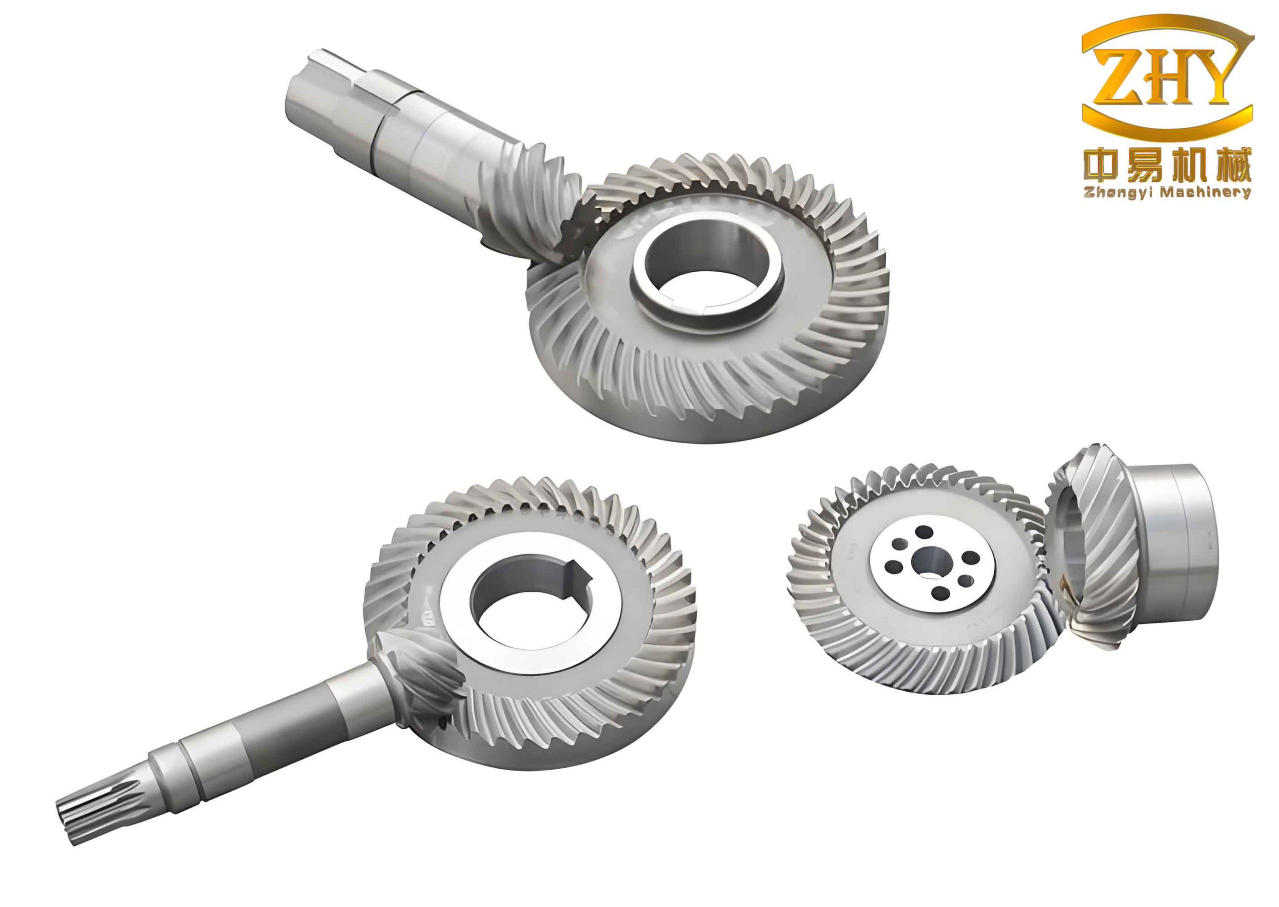
In the field of mechanical transmission, especially in automotive drive axles, hyperboloid gears play a critical role due to their high overlap ratio, smooth operation, and ability to handle offset shafts. However, the complex tooth surfaces of hyperboloid gears pose significant challenges in manufacturing and performance control. The contact pattern between mating gears directly influences vibration, noise, and operational stability, making it essential to analyze and adjust real tooth surfaces based on measurement data. In this article, I will explore a comprehensive methodology for contact analysis and adjustment of hyperboloid gears, leveraging advanced numerical techniques and practical validation. The focus is on reconstructing actual tooth surfaces from measurement points, performing discrete contact analysis, and deriving adjustment parameters to optimize gear performance. Throughout, I will emphasize the application of hyperboloid gears in real-world scenarios, using formulas and tables to summarize key concepts.
Hyperboloid gears, often referred to as hypoid gears, are widely used in vehicles for their efficiency and compact design. The tooth surfaces are generated through complex machining processes, leading to inevitable deviations from theoretical designs due to manufacturing and assembly errors. These deviations affect the contact pattern, which must be controlled to ensure optimal meshing performance. Traditional methods rely on rolling tests to observe contact patterns, but these are time-consuming and may not provide precise adjustment parameters. Therefore, a computational approach based on actual tooth surface measurements is proposed to simulate contact analysis and facilitate machine tool setting corrections. This approach not only reduces reliance on physical trials but also enhances accuracy in hyperboloid gear production.
The core of this methodology involves three main steps: tooth surface fitting using double cubic spline interpolation, discrete contact analysis via a two-dimensional golden section refinement method, and adjustment calculation based on installation distance models. I will detail each step, supported by mathematical formulations and algorithmic flows. Additionally, I will present a case study involving hyperboloid gears from an automobile drive axle, demonstrating the alignment between simulation results and actual rolling tests. By integrating these elements, this article aims to provide a robust framework for engineers and researchers working with hyperboloid gears.
Tooth Surface Measurement and Fitting
Accurate representation of actual tooth surfaces is the foundation for contact analysis of hyperboloid gears. In typical gear measurement centers, tooth surfaces are sampled at grid points—often 5 points along the profile direction and 9 points along the lengthwise direction, resulting in 45 measurement points per tooth. These points capture deviations from the theoretical surface, which are crucial for reconstructing the real geometry. The deviation values, denoted as $\delta_{ij}$, are combined with theoretical surface coordinates to obtain actual surface points. For a given grid point $(i,j)$, where $i$ indexes the profile direction and $j$ indexes the lengthwise direction, the actual position vector $\mathbf{R}_{i,j}$ is computed as:
$$ \mathbf{R}_{i,j} = \mathbf{r}_{i,j} + \delta_{i,j} \cdot \mathbf{n}_{i,j} $$
Here, $\mathbf{r}_{i,j}$ is the theoretical surface position vector, and $\mathbf{n}_{i,j}$ is the unit normal vector at that point. This additive model accounts for manufacturing errors, enabling a precise digital twin of the hyperboloid gear tooth surface.
To facilitate contact analysis, the discrete measurement points are fitted into a continuous surface using double cubic Non-Uniform Rational B-Spline (NURBS) representation. NURBS surfaces offer flexibility and accuracy in modeling complex geometries, making them ideal for hyperboloid gears. The fitted surface $\mathbf{S}(u,v)$ is expressed as:
$$ \mathbf{S}(u,v) = \frac{\sum_{i=0}^{m} \sum_{j=0}^{n} N_{i,3}(u) N_{j,3}(v) w_{i,j} \mathbf{K}_{i,j}}{\sum_{i=0}^{m} \sum_{j=0}^{n} N_{i,3}(u) N_{j,3}(v) w_{i,j}} $$
where $\mathbf{K}_{i,j}$ are control points, $w_{i,j}$ are weight factors, and $N_{i,3}(u)$ and $N_{j,3}(v)$ are cubic B-spline basis functions in the $u$ (lengthwise) and $v$ (profile) directions, respectively. The fitting process involves first computing control points along the profile direction and then along the lengthwise direction, ensuring a smooth representation of the actual tooth surface. This reconstruction is critical for subsequent contact analysis, as it allows interpolation at any point on the surface, not just the measured grid points.
However, the initial grid of 45 points may be insufficient for detailed contact analysis, especially near contact zones where high precision is required. Therefore, a refinement strategy is employed using two-dimensional golden section interpolation. This method divides the surface region into smaller rectangles based on the golden ratio (0.618 and 0.382), iteratively increasing point density until a desired accuracy is achieved. The refined grid enhances the resolution of contact calculations, enabling more accurate determination of meshing points for hyperboloid gears. The process can be summarized in the following table, which outlines the steps for tooth surface fitting and refinement:
| Step | Description | Key Parameters |
|---|---|---|
| 1 | Measure tooth surface deviations at grid points | Grid size: 5×9 points, deviation $\delta_{ij}$ |
| 2 | Compute actual surface points | $\mathbf{R}_{i,j} = \mathbf{r}_{i,j} + \delta_{i,j} \mathbf{n}_{i,j}$ |
| 3 | Fit double cubic NURBS surface | Control points $\mathbf{K}_{i,j}$, weights $w_{i,j}$ |
| 4 | Refine grid using 2D golden section | Golden ratios: 0.618 and 0.382, tolerance $\sigma$ |
| 5 | Validate surface accuracy | Compare with additional measurement points |
This fitting and refinement process ensures that the digital model closely matches the physical hyperboloid gears, setting the stage for reliable contact analysis.
Discrete Tooth Contact Analysis Algorithm
Contact analysis for hyperboloid gears involves simulating the meshing between pinion and gear tooth surfaces under specified assembly conditions. Given the point-contact nature of hyperboloid gears, the goal is to determine the contact path, transmission error, and contact pattern on the actual surfaces. A discrete approach is adopted, where the refined surface points are used to find meshing points iteratively. The algorithm leverages the principle that at a meshing point, the distance between the pinion and gear surfaces is minimized, and the surfaces do not interfere.
The meshing condition can be formulated using coordinate transformations and kinematic constraints. Let $(\mathbf{O}_f: X_f, Y_f, Z_f)$ be a fixed coordinate system, and $(\mathbf{O}_1: X_1, Y_1, Z_1)$ and $(\mathbf{O}_2: X_2, Y_2, Z_2)$ be coordinate systems attached to the pinion and gear, respectively. The position vectors of points on the pinion and gear surfaces are denoted as $\mathbf{r}^1(u_1, v_1, \phi_1)$ and $\mathbf{r}^2(u_2, v_2, \phi_2)$, where $u, v$ are surface parameters and $\phi$ is the rotation angle. To account for assembly adjustments, installation deviations $\Delta V$ (offset distance), $\Delta H$ (pinion axial displacement), and $\Delta J$ (gear axial displacement) are introduced. The meshing equations must satisfy:
$$ \mathbf{r}^1_f(u_1, v_1, \phi_1, \Delta V, \Delta H, \Delta J) = \mathbf{r}^2_f(u_2, v_2, \phi_2) $$
$$ \mathbf{n}^1_f(u_1, v_1, \phi_1, \Delta V, \Delta H, \Delta J) = \mathbf{n}^2_f(u_2, v_2, \phi_2) $$
$$ \frac{\partial \mathbf{r}^1_f}{\partial u_1} \cdot \left( \frac{\partial \mathbf{r}^2_f}{\partial u_2} \times \frac{\partial \mathbf{r}^2_f}{\partial v_2} \right) = 0 $$
$$ \frac{\partial \mathbf{r}^1_f}{\partial v_1} \cdot \left( \frac{\partial \mathbf{r}^2_f}{\partial u_2} \times \frac{\partial \mathbf{r}^2_f}{\partial v_2} \right) = 0 $$
$$ \mathbf{n}^2_f \cdot \mathbf{v}^{12}_f = f(u_1, v_1, \phi_1, u_2, v_2, \phi_2, \Delta V, \Delta H, \Delta J) = 0 $$
Here, $\mathbf{n}_f$ is the unit normal vector in the fixed system, and $\mathbf{v}^{12}_f$ is the relative velocity between the gear surfaces. These equations ensure contact at a point with continuous tangency and no penetration. However, solving this system directly is complex due to the piecewise nature of the NURBS surfaces. Instead, a discrete search method is employed.
The algorithm begins with an initial meshing point, often derived from theoretical contact analysis. Then, for each incremental rotation of the gear, the pinion surface is discretized into a dense grid of points. For each point $\mathbf{P}^{1}_{ij}$ on the pinion, the distance to the gear surface $\mathbf{P}^{2}_{ij}$ is computed as:
$$ D_{p \times q} = | \mathbf{r}^{2}_{f,ij} – \mathbf{r}^{1}_{f,ij} | \quad (i=0,1,\dots,m; j=0,1,\dots,n) $$
The point with the minimum distance is considered a candidate meshing point. To refine accuracy, the two-dimensional golden section method is applied around this candidate. The region is divided into smaller rectangles, and distances are evaluated at their centers iteratively until the region size falls below a tolerance $\sigma$. This process efficiently locates the meshing point without solving nonlinear equations directly.
Interference detection is crucial to ensure valid contact. For any pair of points $\mathbf{P}^{1}_{ij}$ and $\mathbf{P}^{2}_{ij}$, interference occurs if the dot product between the gear surface normal at $\mathbf{P}^{1}_{ij}$ and the vector from $\mathbf{P}^{1}_{ij}$ to $\mathbf{P}^{2}_{ij}$ is negative:
$$ S_{p \times q} = \mathbf{n}^{1}_{f,ij} \cdot (\mathbf{r}^{2}_{f,ij} – \mathbf{r}^{1}_{f,ij}) < 0 $$
If $\min(S_{p \times q}) < 0$, the surfaces interfere, indicating an invalid meshing condition. The algorithm then adjusts the rotation or installation parameters to avoid interference. The overall flowchart for the contact analysis algorithm is summarized below:
| Step | Action | Mathematical Basis |
|---|---|---|
| 1 | Initialize with theoretical meshing point | $\phi_1^0, \phi_2^0$ from design settings |
| 2 | Discretize pinion surface into grid | Grid points $\mathbf{P}^{1}_{ij}$ via NURBS evaluation |
| 3 | Compute distances to gear surface | $D_{p \times q} = | \mathbf{r}^{2}_{f,ij} – \mathbf{r}^{1}_{f,ij} |$ |
| 4 | Find minimum distance point | $\min(D_{p \times q})$ as candidate |
| 5 | Refine using 2D golden section | Divide region by ratios 0.618/0.382, iterate |
| 6 | Check interference condition | $S_{p \times q} = \mathbf{n}^{1}_{f,ij} \cdot (\mathbf{r}^{2}_{f,ij} – \mathbf{r}^{1}_{f,ij})$ |
| 7 | Adjust parameters if interference | Update $\Delta V, \Delta H, \Delta J$ or $\phi$ |
| 8 | Repeat for next rotation increment | Loop until full mesh cycle |
This discrete contact analysis algorithm provides a practical way to simulate the meshing of hyperboloid gears, accounting for actual surface geometries and assembly variations. It outputs the contact path, transmission error curve, and contact pattern, which are essential for performance evaluation.
Adjustment Calculation Model for Contact Pattern Correction
In practice, the contact pattern on hyperboloid gears often deviates from the desired location due to manufacturing tolerances. For instance, the pattern might be biased toward the toe or heel, or toward the top or root of the tooth. To correct this, adjustment parameters for installation distances—specifically, pinion axial displacement $\Delta H$, gear axial displacement $\Delta J$, and offset distance $\Delta V$—are calculated. These adjustments shift the contact pattern to the ideal position, typically near the center of the tooth surface.
The adjustment model is based on the geometry of the gear pair. Let $M_0$ be the ideal contact point on the gear tooth surface, with coordinates $(x^*_2, y^*_2)$ in a local coordinate system $(O_0: X_0, Y_0)$. The actual contact point $M^*$ is displaced by distances $s$ (profile direction) and $t$ (lengthwise direction). The relationship between the 3D surface coordinates $(x_2, y_2, z_2)$ in the gear coordinate system $(O_2: X_2, Y_2, Z_2)$ and the local coordinates is given by:
$$ x_2 \cos \gamma_2 + \sqrt{y_2^2 + z_2^2} \sin \gamma_2 – l_{MD} = x^*_2 + t $$
$$ -x_2 \sin \gamma_2 + \sqrt{y_2^2 + z_2^2} \cos \gamma_2 = y^*_2 + s $$
Here, $\gamma_2$ is the gear pitch cone angle, and $l_{MD}$ is the mean cone distance. These equations link the surface geometry to the contact pattern location. To derive adjustment parameters, the meshing equations from the previous section are solved with the constraint that the backlash remains constant. This constraint ensures that gear pair clearance is preserved during adjustments and is expressed as:
$$ \Delta J + \Delta H \tan \gamma_1 = 0 $$
where $\gamma_1$ is the pinion pitch cone angle. Combining this with the meshing equations results in a system of nine equations with nine unknowns: $u_1, v_1, \phi_1, u_2, v_2, \phi_2, \Delta V, \Delta H, \Delta J$. Due to the complexity of NURBS surfaces, the Newton-Raphson iterative method is used for solution. Let $\mathbf{X} = [u_1, v_1, \phi_1, u_2, v_2, \phi_2, \Delta V, \Delta H, \Delta J]^T$ represent the vector of unknowns, and $f_d(\mathbf{X})$ for $d=1,2,\dots,9$ represent the equations. The Jacobian matrix $\mathbf{F}'(\mathbf{X}^k)$ is computed at each iteration $k$, and the update is:
$$ \mathbf{X}^{k+1} = \mathbf{X}^k – \mathbf{F}'(\mathbf{X}^k)^{-1} \mathbf{f}(\mathbf{X}^k) $$
The iteration continues until $||\mathbf{X}^{k+1} – \mathbf{X}^k|| < \sigma$, where $\sigma$ is a convergence tolerance. This yields the adjusted parameters that move the contact pattern to the desired location. These parameters can then be converted into machine tool setting corrections, such as changes in cutter position or machine axes, enabling precise manufacturing of hyperboloid gears.
To illustrate the adjustment process, consider a scenario where the contact pattern is biased toward the toe (large end) of the gear tooth. The displacement $t$ might be positive, indicating a need to shift the pattern toward the heel. The adjustment calculation would output specific values for $\Delta V, \Delta H, \Delta J$, which can be tabulated for different hyperboloid gear designs. The following table provides an example of adjustment parameters for various contact pattern deviations:
| Deviation Type | Displacement $s$ (mm) | Displacement $t$ (mm) | $\Delta V$ (mm) | $\Delta H$ (mm) | $\Delta J$ (mm) |
|---|---|---|---|---|---|
| Toe bias | 0 | +7.0 | +0.312 | -0.433 | +0.062 |
| Heel bias | 0 | -5.0 | -0.223 | +0.310 | -0.044 |
| Top bias | +1.0 | 0 | +0.150 | -0.208 | +0.030 |
| Root bias | -1.5 | 0 | -0.225 | +0.312 | -0.045 |
These values are derived from the mathematical model and can be validated through simulation or rolling tests. By applying such adjustments, manufacturers can optimize the performance of hyperboloid gears, reducing noise and improving durability.
Case Study: Application to Automobile Drive Axle Hyperboloid Gears
To demonstrate the practicality of the proposed methodology, I applied it to a hyperboloid gear pair from an automobile drive axle. The basic parameters of the gear set are listed in the table below, which includes key dimensions and geometric properties essential for hyperboloid gears analysis.
| Parameter | Pinion | Gear |
|---|---|---|
| Number of teeth | 8 | 39 |
| Module (mm) | 4.611 | – |
| Face width (mm) | 25 | 30 |
| Offset distance (mm) | 25 | 25 |
| Outer diameter (mm) | 56.73 | 171.05 |
| Spiral angle | 50° | – |
| Pitch cone angle | 14°11′ | 30°41′ |
| Face cone angle | 18°10′ | 76°49′ |
| Root cone angle | 11°37′ | 70°48′ |
| Hand of spiral | Left | Right |
The tooth surfaces were measured on a gear measurement center, resulting in deviation maps for both pinion and gear. Using the double cubic NURBS fitting, actual surfaces were reconstructed. The discrete contact analysis algorithm was then implemented, with a refinement tolerance of $\sigma = 0.001$ mm. The initial contact pattern from simulation showed a bias toward the toe of the gear convex side, with displacements $s = 1$ mm and $t = 7$ mm from the ideal center. This aligned with observations from preliminary rolling tests, indicating the need for adjustment.
Applying the adjustment calculation model, the derived parameters were $\Delta V = 0.312$ mm, $\Delta H = -0.433$ mm, and $\Delta J = 0.062$ mm. These were used to modify the virtual assembly in the simulation. After adjustment, the contact pattern shifted toward the center, as shown in the transmission error and contact pattern plots. The transmission error, which indicates meshing smoothness, was computed as the difference between actual and theoretical rotation angles:
$$ \Delta \phi = \phi_2 – \frac{N_1}{N_2} \phi_1 $$
where $N_1$ and $N_2$ are tooth numbers. The adjusted case showed reduced fluctuation in $\Delta \phi$, suggesting improved performance for hyperboloid gears.
To validate the simulation, physical rolling tests were conducted on a CNC rolling tester. The contact pattern before adjustment indeed appeared near the toe, while after implementing the machine tool corrections based on $\Delta V, \Delta H, \Delta J$, the pattern moved to the center. This correlation between simulation and experiment confirms the accuracy of the methodology. The entire process, from measurement to adjustment, highlights the value of computational tools in optimizing hyperboloid gears, reducing trial-and-error in manufacturing.
Furthermore, sensitivity analysis can be performed to understand how variations in installation parameters affect the contact pattern. For hyperboloid gears, small changes in offset or axial positions can lead to significant shifts in contact, underscoring the importance of precise adjustment. The table below summarizes the sensitivity coefficients for this case study, derived from partial derivatives of the contact position with respect to $\Delta V, \Delta H, \Delta J$:
| Parameter | Sensitivity in $s$ (mm/mm) | Sensitivity in $t$ (mm/mm) |
|---|---|---|
| $\Delta V$ | 0.48 | 0.32 |
| $\Delta H$ | -0.67 | 0.45 |
| $\Delta J$ | 0.10 | -0.07 |
These coefficients indicate that $\Delta H$ has the greatest influence on the profile direction shift $s$, which is typical for hyperboloid gears due to their conical geometry. Such insights aid in fine-tuning adjustments during production.
Conclusion
In this article, I have presented a comprehensive approach for actual tooth surface contact analysis and adjustment calculation of hyperboloid gears. The methodology integrates tooth surface measurement, NURBS-based fitting, discrete contact analysis using two-dimensional golden section refinement, and mathematical modeling for installation adjustments. By focusing on hyperboloid gears, which are pivotal in automotive and industrial applications, this work addresses the challenge of controlling contact patterns to enhance gear performance. The proposed algorithm effectively simulates meshing behavior, providing transmission error curves and contact patterns that align with physical rolling tests.
The key advantages of this approach include reduced reliance on empirical trials, improved accuracy through digital surface reconstruction, and the ability to derive precise machine tool corrections. The case study on automobile drive axle gears demonstrated the practicality of the method, with simulation results matching experimental outcomes after adjustment. Future work could extend this methodology to include dynamic load conditions, thermal effects, or more complex surface modifications for hyperboloid gears. Additionally, integration with machine learning could automate the adjustment process further, optimizing hyperboloid gears production in real-time.
Overall, the techniques described here offer a robust framework for engineers and researchers working with hyperboloid gears, enabling better design, manufacturing, and performance optimization. As industries demand higher efficiency and quieter transmissions, such computational tools will become increasingly valuable in the advancement of gear technology.